In my previous post I tried to get clear about when variables could be safely removed from a causal model without affecting what the model is capable of telling us about singular causal relations. There, I endorsed two principles stating when causal models may be reduced by excising variables in a particular way. If we endorse these principles, and we want to give a theory of singular causation formulated in terms of correct causal models, then we should want that theory to give the very same verdicts before and after model reduction. The point of today’s post is that there is a wide family of theories of causation which run afoul of this constraint. Those theories will say that two variable values are causally related in one model, but reverse this judgment when the model is reduced.
1. Counterfactual Counterfactual Theories of Singular Causation
1.1 Counterfactuals in Causal Models
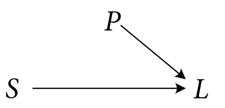
Causal models allow us to evaluate certain causal counterfactual conditionals. For instance, recall the causal model describing the relations of causal determination between whether the switch is up, whether the power is on, and whether the light is illuminated.
$$
\begin{aligned}
L &:= S \wedge P \\\
P &:= S
\end{aligned}
$$
Suppose that, actually, the switch is down, $S=1$, so that the power is on and the light is illuminated. If we want to evaluate the counterfactual conditional $P = 0 \hspace{4pt}\Box\hspace{-4pt}\to L = 1$ (were the power off, the light would be illuminated), we mutilate the model $\mathbb{M}$ by removing $P$'s equation, severing $P$'s dependence upon $S$, and setting its value to $0$ directly. That is, we exogenize the variable $P$, and add the assignment $P=0$ to the context $\vec{u}$. Graphically, we cut the arrow going into $P$, but leave all other arrows intact.
Call the resulting mutilated model “$\mathbb{M}[P \to 0]$”. The semantics for counterfactuals tells us that $P = 0 \hspace{4pt}\Box\hspace{-4pt}\to L = 1$ is true in the model $\mathbb{M}$ iff $L=1$ is true in the mutilated model $\mathbb{M}[P \to 1]$.
$$
\mathbb{M} \models P = 0 \hspace{4pt}\Box\hspace{-4pt}\to L = 1 \quad \iff \quad \mathbb{M}[P \to 0] \models L =1
$$
Since $L=0$ in the mutilated model $\mathbb{M}[P \to 0]$, this tells us that the counterfactual $P = 0 \hspace{4pt}\Box\hspace{-4pt}\to L = 1$ is false in the original model $\mathbb{M}$.
More generally, if $\vec{X}$ is a vector of variables in $\mathbb{U} \cup \mathbb{V}$ and $\vec{x}$ is some assignment of values to those variables, then we may define $\mathbb{M}[\vec{X} \to \vec{x}]$ to be the mutilated model that you get by going through each variable $ X \in \vec{X}$ and, if $X$ is endogenous, removing $X$'s structural equation $\phi_X$ from $\mathbb{E}$, moving $X$ from $\mathbb{V}$ to $\mathbb{U}$, and adding the assignment $\vec{x}(X)$ to the context $\vec{u}$. (By the way, “$\vec{x}(X)$” is the value which $\vec{x}$ assigns to the variable $X$.) On the other hand, if $X \in \vec{X}$ is exogenous, then you simply change the context so that $\vec{u}(X) = \vec{x}(X)$. Then, for any $\phi$, we have that
$$
\mathbb{M} \models \vec{X} = \vec{x} \hspace{4pt}\Box\hspace{-4pt}\to \phi \quad\iff \quad \mathbb{M}[\vec{X} \to \vec{x}] \models \phi
$$
1.2 Counterfactual Counterfactual Depdendence
Many contemporary theories of causation fit into the following general schema, which we can call “Counterfactual Counterfactual":
Counterfactual Counterfactual. $C=c$ caused $E=e$ in causal model $\mathbb{M}$ iff there is some value of $C$, $c'$, such that
$$
\mathbb{M}[\vec{G}\to\vec{g}] \models C = c’ \hspace{4pt}\Box\hspace{-4pt}\to E \neq e
$$
for some suitable vector of variable $\vec{G}$ and a suitable assignment of values $\vec{g}$.
According to Counterfactual Counterfactual, causation is not counterfactual dependence; rather, it is counterfactual dependence in some counterfactual scenario, $\vec{G} = \vec{g}$. Assuming that the empty vector of variables counts as suitable, Counterfactual Counterfactual will entail that counterfactual dependence is sufficient for causation.
We will get different theories of causation depending upon which vectors of variables, and which assignments of values, we take to be suitable. For instance, the account of Hitchcock (2001) tells us that $\vec{G}$ and $\vec{g}$ are suitable iff, in $\mathbb{M}$, there is some directed path leading from the variable $C$ to the variable $E$, $C \to V_1 \to V_2 \to \dots \to V_N \to E$, such that, in the counterfactual model $\mathbb{M}[\vec{G} \to \vec{g}]$, every variable $V$ along this path retains its actual value in the original model, $\vec{u}(V)$.
Hitchcock (2001). $\vec{G}$ and $\vec{g}$ are suitable iff there some some path from $C$ to $E$ such that, for every variable $V$ along this path,
$$
\mathbb{M}[\vec{G} \to \vec{g}] \models V = \vec{u}(V)
$$
There are some cases in which Hitchcock looks too strong (e.g., the Voting Machine case from appendix A.2 of Halpern & Pearl (2005)). These and other cases were taken to motivate a move to the following weaking.
Halpern and Pearl (2005). $\vec{G}$ and $\vec{g}$ are suitable iff, for all vectors of variables $\vec{P}$ not in $\vec{G}$, and any subvector $\vec{H}$ of $\vec{G}$,
$$
\mathbb{M}[\vec{H} \to \vec{g}(\vec{H}), \vec{P} \to \vec{u}(\vec{P}), C \to c] \models E=e
$$
Notice that, if a counterfactual setting $\vec{G} = \vec{g}$ is suitable according to Hitchcock (2001), then it will automatically be suitable according to Halpern and Pearl (2005). So, if $C=c$ caused $E=e$ according to Hithcock (2001), then $C=c$ caused $E=e$ according to Halpern and Pearl (2005).
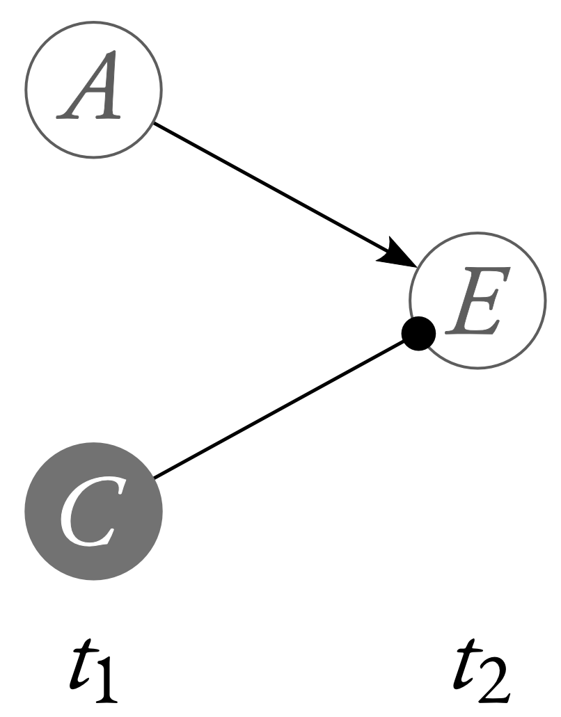
Both of these accounts of causation face a problem with cases of what’s come to be known as bogus prevention, illustrated by the neuron diagram below.
In this neuron diagram, $C$'s firing does not prevent $E$ from firing (that is: $C$'s firing did not cause $E$ to not fire). However, both Hitchcock (2001) and Halpern and Pearl (2005) get the verdict that $C$'s firing prevented $E$ from firing. That’s because both of them rule the singleton vector of variables $\vec{G} = (A)$, with the assignment $\vec{g}=1$, suitable. And, in this counterfactual setting, whether $E=0$ counterfactually depends upon whether $C = 1$.
In response to cases like these, there has been further emendation of the Halpern and Pearl account to incorporate standards of normality, or typicality. Halpern (2008) emends the Halpern and Pearl (2005) account like so:
Halpern (2008). $\vec{G}$ and $\vec{g}$ are suitable iff, for all vectors of variables $\vec{P}$ not in $\vec{G}$, and any subvector $\vec{H}$ of $\vec{G}$,
$$
\mathbb{M}[\vec{H} \to \vec{g}(\vec{H}), \vec{P} \to \vec{u}(\vec{P}), C \to c] \models E=e
$$
and, in addition, there is some assignment of values to the variables in the model such that, in that assignment, $\vec{G} = \vec{g}$ and $C = c'$, and that assignment is at least as normal, or typical as the variable assignment of the original model $\mathbb{M}$.
This definition requires us to outfit our causal models with a ranking over assignments of values to all of the variables in $\mathbb{U} \cup \mathbb{V}$. There will be complicated questions about which variable values are more normal than which others; however, it we restrict our attention to simple neuron diagrams, we can at least rest assured that everybody seems to agree that it is more normal or typical for a neuron to not fire than it is for it to fire. If we assume that $A$'s not firing is more normal that $A$'s firing, then Halpern (2008) tells us that the counterfactual setting $A=1$ in Bogus Prevention is not suitable; and, therefore, that $C=1$ did not cause $E=1$.
Notice that, if a counterfactual setting $\vec{G} = \vec{g}$ is suitable according to Halpern (2008), then it will automatically be suitable according to Halpern and Pearl (2005). So, if $C=c$ caused $E=e$ according to Halpern (2008), then $C=c$ caused $E=e$ according to Halpern and Pearl (2008).
2.Counterfactual Counterfactual Accounts Reverse Causal Judgments in Model Reductions
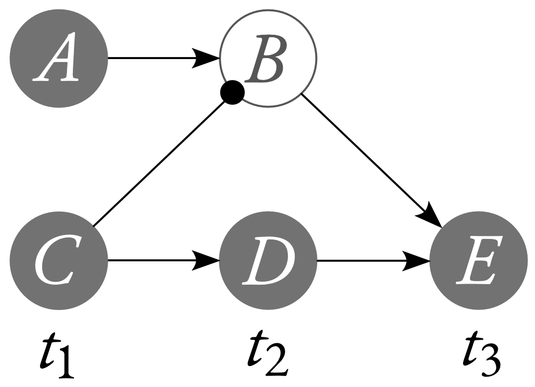
Recall the Lewisian neuron diagram of a case of preemption.
We may model this neuron diagram with the following system of structural equations (where the variables have the natural interpretation, with $1$ corresponding to firing and $0$ corresponding to not firing):
$$
\begin{aligned}
E &:= B \vee D \\\
D &:= C \\\
B &:= A \wedge \neg C
\end{aligned}
$$
(The context is just $C=1$ and $A=1$.) Let’s call this model “$\mathbb{M}$”. In the original neuron diagram, $C$'s firing is a cause of $E$'s firing. So we should want our theory of singular causation to tell us that, in this causal model, $C=1$ is a cause of $E=1$. Getting cases like this right is non-negotiable for a theory of singular causation. And, fortunately, counterfactual counterfactual accounts like Hitchcock’s (2001) and Halpern and Pearl’s (2005) are capable of saying that $C=1$ is a cause of $E=1$ in the causal model above. To deliver this verdict, those theories let $\vec{G} = (B)$, with $\vec{g} = (0)$. As you may verify for yourself, Hitchcock (2001), Halpern and Pearl (2005), and Halpern (2008) all deem this choice suitable. But then,
$$
\mathbb{M}[B \to 0] \models C = 0 \hspace{4pt}\Box\hspace{-4pt}\to E = 0
$$
That is: in the counterfactual scenario where $B$'s value is held fixed at $0$, had $C$ not fired, $E$ would not have fired either. So, Counterfactual Counterfactual deems $C=1$ a cause of $E=1$.
Note that the following is an exogenous reduction of this model in which we have excised the exogenous variable $A$ by substituting $1$ for $A$ in $B$'s structural equation.
$$
\begin{aligned}
E &:= B \vee D \\\
D &:= C \\\
B &:= \neg C
\end{aligned}
$$
Call the resulting model “$\mathbb{M}_A$”. The endogenous variable set of $\mathbb{M}_A$ is non-empty and the equation for $B$ is still surjective, so this is a valid exogenous reduction. By our principle Valid Exogenous Reduction Preserves Correctness (see the previous post), $\mathbb{M}_A$ is correct if the original model $\mathbb{M}$ was.
Given $\mathbb{M}_A$, we may excise the endogenous variable $B$ by removing $B$'s structural equation and substituting $\neg C$ for $B$ in $E$'s structural equation.
$$
\begin{aligned}
E &:= \neg C \vee D \\\
D &:= C
\end{aligned}
$$
Call the resulting model “${\mathbb{M}_A}_B$”. $B$ is not a collider in $\mathbb{M}_A$, so this is a valid endogenous reduction of $\mathbb{M}_A$. By our principle Valid Endogenous Reduction Preserves Correctness (see the previous post), ${\mathbb{M}_A}_B$ is correct if $\mathbb{M}_A$ was.
However, just considering this model, Counterfactual Counterfactual tells us that $C=1$ is not cause of $E=1$. For the only possible choices of $\vec{G}$ are the empty vector and the singleton vector $(D)$. Since $E=1$ does not counterfactually depend upon $C=1$, the empty vector does not witness $C=1$'s causing $E=1$. And
$$
{\mathbb{M}_A}_B[D \to 1] \models C=0 \hspace{4pt}\Box\hspace{-4pt}\to E=1
$$
So there is no counterfactual dependence between $E=1$ and $C=1$ in the counterfactual scenario in which $D$ is held fixed at $1$. And
$$
{\mathbb{M}_A}_B[D \to 0] \models C=0 \hspace{4pt}\Box\hspace{-4pt}\to E=1
$$
So there is no counterfactual dependence between $E=1$ and $C=1$ in the counterfactual scenario in which $D$ is held fixed at $0$. So there is no counterfactual dependence between $E=1$ and $C=1$ period. So they are not causally related, according to Counterfactual Counterfactual.
What we’ve just seen is that, if we accept the principles on valid model reduction from the previous post, then the verdicts of a theory like Counterfactual Counterfactual vary from correct model to correct model. Above, we relied upon both the principle Valid Exogenous Reduction Preserves Correctness and Valid Endogenous Reduction Preserves Correctness. However, we can get Halpern (2008) to flip its verdict by just excising an exogenous variable from a correct causal model.
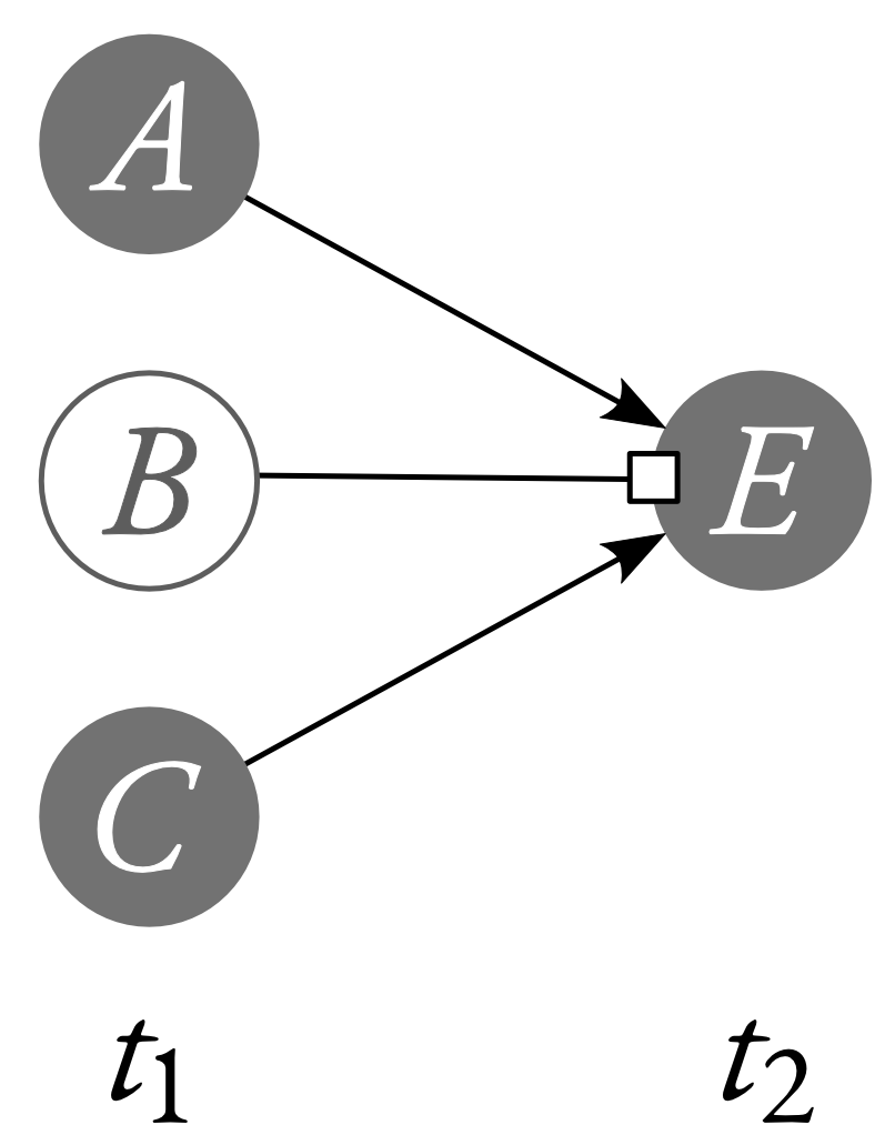
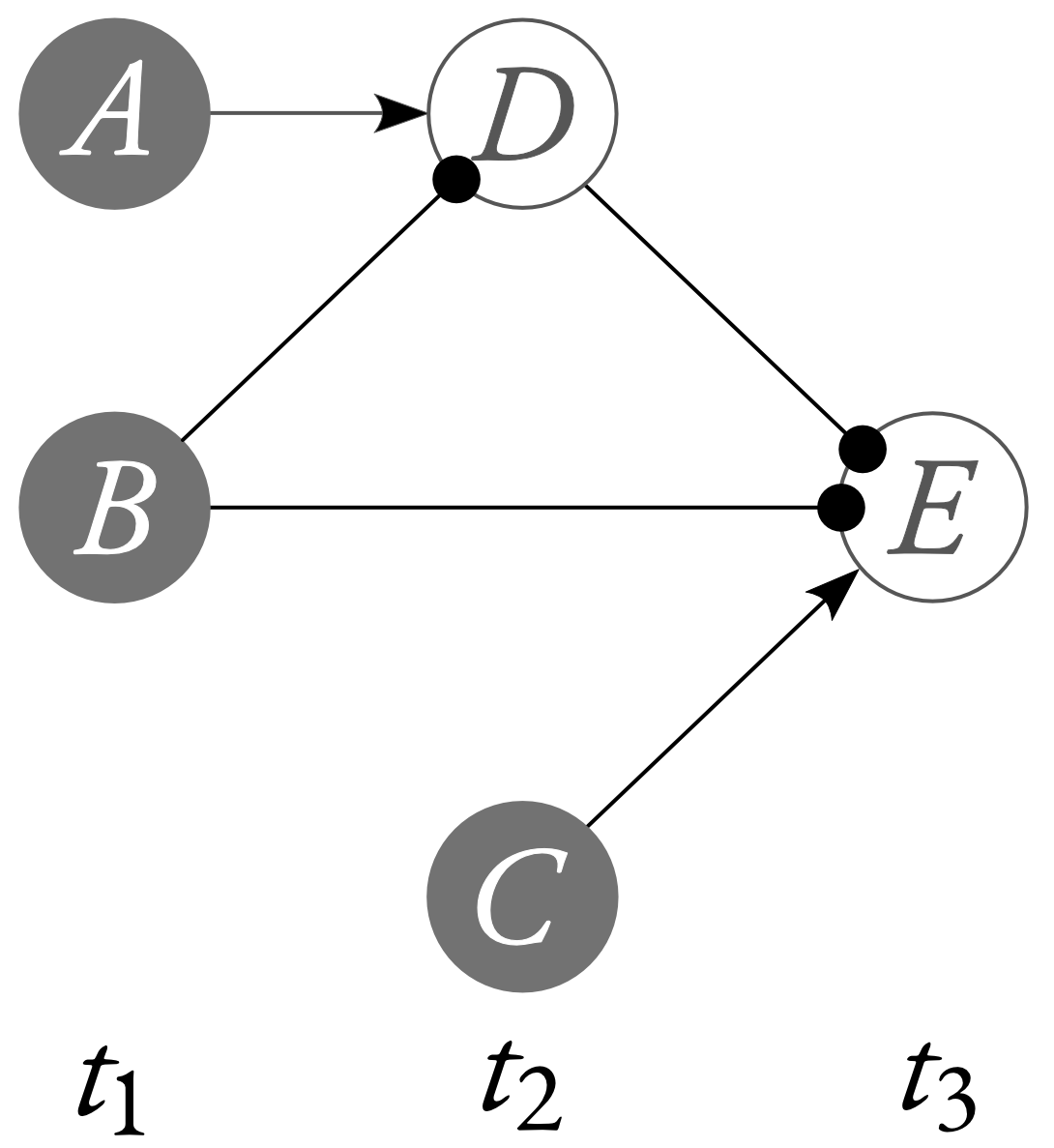
Consider the following neuron diagram.
Here’s how to read this diagram: if $B$ fires at $t_1$, then it will cancel out any one signal sent from $A$ or $C$. So, if $B$ fires and exactly one of $A$ and $C$ fire, then $E$ will not fire. If $B$ fires and both $A$ and $C$ fire, then $E$ will fire. And, if $B$ doesn’t fire, then $E$ will fire iff at least one of $A$ and $C$ fire.
We can represent this neuron diagram with the following structural equation.
$$
E := (\neg B \wedge (A \vee C)) \vee (B \wedge (A \wedge C))
$$
(The context is $A=C=1$ and $B=0$.) Call the causal model containing these variables, this context, and this equation “$\mathbb{M}$”. Given given the natural assumption that not firing is more normal, or typical, than firing, Halpern (2008) tells us that $C$'s firing ($C=1$) is a cause of $E$'s firing ($E=1$) in $\mathbb{M}$. That’s because the variable assignment in which none of the neurons fire is more normal that the actual variable assignment, and this is an assignment in which $A=C=0$. So, Halpern (2008) tells us that the counterfactual setting $A=0$ is suitable; and, in this counterfactual setting, whether $E=1$ counterfactually depends upon whether $C=1$.
$$
\mathbb{M}[A=0] \models C = 0 \hspace{4pt}\Box\hspace{-4pt}\to E = 0
$$
So, $C=1$ caused $E=1$. Now, I don’t think that this verdict is a desideratum of a theory of causation. I, like Lewis and Mackie, am content with an account which says that, while neither $A=1$ nor $C=1$ individually caused $E=1$, the disjunction (or the fusion, or what-have-you) of $A=1$ and $C=1$ did. However, I am also content with an account according to which $C=1$ was a cause of $E=1$. And that is how Halpern (2008), like Hitchcock (2001) and Halpern and Pearl (2005), comes down on this case.
Suppose that we excise the exogenous variable $A$ from this model. This gives us the new model $\mathbb{M}_A$, which contains the variables $C, B,$ and $E$, the structural equation
$$
E := \neg B \vee C
$$
The resulting endogenous variable set is non-empty, and the resulting structural equation is surjective, so this exogenous reduction is valid. By our principle Valid Exogenous Reduction Preserves Correctness, $\mathbb{M}_A$ is correct if $\mathbb{M}$ was.
Now, while Halpern (2008) said that $C=1$ caused $E=1$ in $\mathbb{M}$, it reverses this judgment in $\mathbb{M}_A$. That’s because, in the actual context $B=0$, whether $E=1$ does not counterfactually dependend upon whether $C=1$. And while, in the counterfactual setting $B=1$, whether $E=1$ does counterfactually depend upon whether $C=1$,
$$
\mathbb{M}_A[B \to 1] \models C=0 \hspace{4pt}\Box\hspace{-4pt}\to E=0
$$
This counterfactual setting is not suitable, according to Halpern (2008). For having $B$ fire is less normal than having $B$ not fire. (Or, if we reject this normality ranking, for whatever reason, this calls into question whether the account is capable of getting the right verdict in Bogus Prevention.)
So, again, if we accept the principle that Valid Exogenous Reduction Preserves Correctness, then the verdicts of Halpern (2008) vary from correct model to correct model.
2017, Oct 1
when can variables be safely removed from a causal model?
Much of our causal talk consists of sentences of the form “c caused e”, where both c and e are token, non-repeatable events or facts or what-have-you (there will be disagreement about what kinds of things ‘c’ and ‘e’ denote, but for now, I’ll just call them ‘events’). Let’s call the kinds of causal relations we’re talking about with sentences like those ‘singular causal relations’. The topic of causation is not exhausted by singular causal relations. There are other interesting causal notions which are clearly distinct from (though they may bear interesting relations to) singular causation. For instance, “Smoking causes cancer” is not a singular causal claim, but rather a general causal claim, relating not token events but rather general types of events.
Many have become convinced that the best way to theorize about singular causation is by understanding it withing the context of some explicitly represented system of causal determination. Causal determination is a third causal notion, distinct from both singular and general causation. Even though it is incorrect to say that the power being on caused the light to not be illuminated, it is nevertheless true that whether the light is illuminated is causally determined by whether the power is on and the switch is up. And, though one could infer that the power is on from the fact that the light is illuminated, it would be incorrect to say that the whether the power is on is causally determined by whether the light is illuminated. To say this would be to get the direction of causal determination the wrong way ‘round.
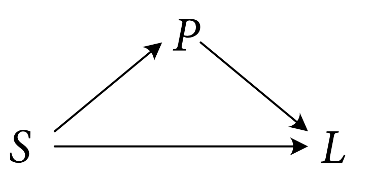
Those who think that systems of causal determination have an important role to play in a theory of singular causation typically think that these systems of causal determination may be represeted with systems of structural equations. A system of structural equations is a particular kind of model of a network of causal determination. The model consists of a vector of variables (see section 1 of this post for more on how to think about variables), together with a vector of structural equations. For instance, we may introduce a variable $P$ for whether the power is on (at the relevant place and the relevant time). This variable takes on the value $1$ if the power is on, takes on the value $0$ if the power is off, and is undefined otherwise. We may similarly introduce a variable $L$ for whether the light is illuminated—a variable which takes on the value $1$ if the light is illuminated, takes on the value $0$ if the light is not illuminated, and takes on the value $0$ otherwise (if, e.g., the light doesn’t exist). And we may introduce a variable $S$ for whether the switch is up or not (again, $1$ if it’s up, $0$ if it’s down, undefined otherwise). A structural equation then tells us how the value of $L$ is causally determined by the values of $P$ and $S$. In particular, it tells us that
\begin{equation}
L := P \wedge S \label{1}\tag{1}
\end{equation}
(Here, “$\wedge$” is just the truth-function ‘and’.) So, $L$ will take on the value $1$ iff both $P$ and $S$ take on the value $1$. If either $P$ or $S$ is $0$, then $L$ will take on the value $0$ as well. When we combine multiple strutctural equations, we can get a system of structural equations. These systems of equations represent networks of causal determination out in the world. For instance, suppose that whether the power is on is structurally determined by whether the light switch is up. If the light switch is up, then the power is on, and if the light switch is down, then the power is off.
\begin{equation}
P := S \tag{2}\label{2}
\end{equation}
Combining the structural equations \eqref{1} and \eqref{2} gives us a system of structural equations
\begin{aligned}
L &:= P \wedge S \\\
P &:= S
\end{aligned}
What makes this system of equations structural is that we are interpreting them causally. The equations don’t just say that there is a certain relationship between the values of $L, P,$ and $S$. They additionally says that the value of $L$ is causally determined by the values of $P$ and $S$; and that the value of $P$ is causally determined by the value of $S$. It is for this reason that I use the asymmetric relation “$:=$”, and not the symmetric relation “$=$”. For instance, it follows from the system of equations consisting of \eqref{1} and \eqref{2} that $S=1$ iff $L=1$; so the equation
$$
S = L
$$
will be true if the system of strutural equations $($\eqref{1}, \eqref{2}$)$ is. However, it will be false that
$$
S := L
$$
For, even though the value of $S$ must match the value of $L$, it is not the case that the value of $S$ is causally determined by the value of $L$. It is this additional information which is conveyed by the symbol $:=$.
In a structural equation, there is exactly one, dependent variable on the left-hand-side of the equation, and at least one independent variable on the right-hand-side. I’ll use “$\mathbf{PA}(V)$” to represent a vector of the independent variables on the right-hand-side of $V$'s structural equation. (It is common to refer to these variables as $V$'s causal parents.) Then, a structural equation is of the form
$$
V := \phi_V(\mathbf{PA}(V))
$$
where $\phi_V$ is some function from the values of the variables in $\mathbf{PA}(V)$ to the values of $V$. I will insist, by the way, that $\phi_V$ be surjective if we are to interpret it causally. I will use “$\phi_V$” to represent the entire structural equation $V := \phi_V(\mathbf{PA}(V))$. If a variable appears on the left-hand-side of a structural equation, then that variable is endogenous. Otherwise, it is exogenous.
What I will call a causal model, $\mathbb{M}$, consists of a vector of exogenous variables $\mathbb{U}$, a vector of endogenous variables $\mathbb{V}$, a vector of structural equations $\mathbb{E}$, and a context, $\vec{u}$, which is an assignment of values to the exogenous variables in $\mathbb{U}$.
Causal Model A causal model $\mathbb{M}$ is a 4-tuple
$$
\mathbb{M} = \langle \mathbb{U}, \mathbb{V}, \mathbb{E}, \vec{u} \rangle
$$
of
A (non-empty) vector $\mathbb{U}$ of exogenous variables, $( U_1, U_2, \dots, U_M )$.
A (non-empty) vector $\mathbb{V}$ of endogenous variables, $ ( V_1, V_2, \dots, V_N)$.
A vector $\mathbb{E}$ of structural equations, $ ( \phi_1, \phi_2, \dots, \phi_N) $, one for each endogenous variables $V_i \in \mathbb{V}$.
A context $\vec{u} = ( u_1, u_2, \dots, u_M )$, which assigns a value to each exogenous variable $U_i \in \mathbb{U}$.
(This is a slightly non-standard presentation. Normally, the context is not taken to be a part of the causal model.)
Given a causal model, we may generate a causal graph by creating a node for every variable and placing an arrow (a directed edge) between two variables $U$ and $V$, with its tail at $U$ and its head at $V$, $U \to V$, iff $U$ appears on the right-hand-side of $V$'s structural equation. For instance, the causal model of the light, the power, and the switch, determines this causal graph:
For a more careful and thorough introduction to causal models, and a theory of when they are correct—that is, when they correctly represent relations of causal determination out in the world—see section 2 of this paper.
When Removing Exogenous Variables Preserves Correctness
Suppose that we have the causal model introduced above, with the context $S=1$ (the switch is actually up). It appears that we can excise the exogenous variable $S$ from this model entirely. We may simply take $S$'s actual value $1$ and plug it into all the structural equations in which the variable $S$ appeared. When we do this, the structural equation associated with $P$ no longer depends upon any variables, and simply says that $P := 1$. That is: the effect of removing the exogenous variable $S$ has been to render $P$ exogenous. And, when we remove the exogenous $S$, the structural equation associated with $L$ becomes $L := P \wedge 1$, or just $L := P$.
We therefore get the causal model $\mathbb{M}$ with the exogenous variable $S$ excised. This is
$$
\mathbb{M}_{S} = \langle (P), (L), (L := P), (1) \rangle.
$$
That is: $\mathbb{M}_S$ consists of the vector of exogenous variables $\mathbb{U} = (P)$, the vector of endogenous variables $\mathbb{V}=(L)$, the vector of structural equations $\mathbb{E} = (L := P)$, and the exogenous assignment $\vec{u} = (1)$ to $P$.
I think that, if the original model $\mathbb{M}$ was correct, then so too is $\mathbb{M}_S$. This follows from a counterfactual understanding of what makes a causal models correct, since the counterfactuals entailed by the new model $\mathbb{M}_S$ are a proper subset of the counterfactuals entailed by the old model $\mathbb{M}$. Given some plausible assumptions, it also follows from my own preferred way of understanding what makes a causal model correct.
No causal model represents all of the features of reality which could potentially make a difference with respect to the values of the variables in the model. In every causal model, we will be taking for granted certain features of, or causal precursors to, the system being modeled. If I want to model the causal determinants of the forest fire, I needn’t explicitly include a variable for the presense of oxygen. So long as there is plenty of oxygen in the atmosphere, it may be true that whether there is a fire is causally determined by whether the lightning struck. Similarly, so long as the light switch is actually up, whether the light is illuminated is causally determined by whether the power is on or off.
In general, if $U$ is an exogenous variable in the causal model $\mathbb{M}$, we can define the $U$-reduction of $\mathbb{M}$ to be what you get when you remove $U$ from $\mathbb{U}$, put into $\mathbb{U}$ any variables in the model which were causally determined by $U$ alone (and remove those variables from $\mathbb{V}$), replace $U$ for its value in the context $\vec{u}$ within every equation in $\mathbb{E}$ (except, of course, for those endogenous variables $V$ which were causally determined by $U$ alone), and update the context $\vec{u}$ appropriately.
Exogenous $U$-Reduction. Given a causal model $\mathbb{M} = \langle \mathbb{U, V, E}, \vec{u} \rangle$, and some $U \in \mathbb{U}$, the $U$-reduction of $\mathbb{M}$, $\mathbb{M}_U$, is $\langle \mathbb{U}_U, \mathbb{V}_U, \mathbb{E}_U, \vec{u}_U \rangle$, where
$\mathbb{U}_U$ is the vector of previously exogenous variables, minus $U$, and plus any endogenous variables whose values were determined by $U$ alone.
$\mathbb{V}_U$ is the vector of previously endogenous variables, minus any whose values were determined by $U$ alone.
$\mathbb{E}_U$ is a vector of structural equations. For each endogenous variable $V$ in $\mathbb{V}_U$, there is exactly one structural equation, which is the result of taking $V$'s old structural equation in $\mathbb{E}$, and replacing the variable $U$ wherever it appears (if at all) with $U$'s value in the context $\vec{u}$
$\vec{u}_U$ is an assignment of values to the variables in $\mathbb{U}_U$ which matches $\vec{u}$ for all exogenous variables previously in $\mathbb{U}$; for those newly exogenous variables, $V$, the assignment in $\vec{u}_U$ is the one determined by taking $V$'s old structural equation in $\mathbb{E}$ and replacing the variable $U$ with $U$'s value in the old context $\vec{u}$.
However, while we can safely remove the exogenous variable $S$ from $\mathbb{M}$ in the context $S=1$, we cannot remove $S$ in the context $S=0$. If we try to do so, we will end up with the structural equation $L := P \wedge 0$. But this equation tells us that $L$'s value does not depend upon $P$'s value. No matter what value $P$ takes on, $L$ will take on the value $0$. So the resulting model would say, falsely, that there $P$ does not causally determine $L$.
The right way to think about this, I believe, is that some $U$-reductions will lead to models which violate necessary conditions on the correctness of causal models. In particular, in order for a structural equation $\phi_V$ to be correct, every value of the right-hand-side variable $V$ must be in the image of $\phi_V$. That is to say: only surjective functions may appear in correct structural equations. And, in order for a causal model to be correct, all of the structural equations it contains must be correct. So, in the context $S=0$, removing the exogenous variable $S$ renders the structural equation $L := P \wedge 0$ non-surjective. Such $U$-reductions are not valid.
Similarly, in order for a causal model to be correct, the vector of endogenous variables $\mathbb{V}$ must be non-empty. Some $U$-reductions will violate this necessary condition on correctness. For instance, consider the $S$-reduced model discussed above. If we try to $U$-reduce this model by excising the exogenous variable $P$, the resulting model, $\mathbb{M}_{S, P}$, will have no endogenous variables. $U$-reductions like these are not valid, either.
In general, we may say that a $U$-reduction is valid iff (1) the resulting endogenous variable set is non-empty, and (2) the resulting structural equations are all surjective.
If a $U$-reduction is valid, then the $U$-reduced model is correct if the original model was. Valid $U$-reduction preserves correctness.
Valid Exogenous Reduction Preserves Correctness. If $\mathbb{M}$ is a correct causal model, and $\mathbb{M}_U$ is a valid exogenous $U$-reduction of $\mathbb{M}$ (i.e., if $\mathbb{M}_U$ is both correct and a $U$-reduction of $\mathbb{M}$), then $\mathbb{M}_U$ is a correct causal model, too.
I have previously laid down conditions for the correctness of causal models. Valid $U$-Reduction Preserves Correctness is not intended as a conjecture about those correctness conditions. I know that my account, as it stands now, violates this principle (the curious may consider the $H$-reduction of the causal model in figure 8 of that paper). Valid $U$-Reduction Preserves Correctness is intended to supplement that account. The principle allows you to move from the correctness of one causal model to the correctness of a certain sub-model, even if the sub-model was not previously deemed correct on its own.
When Removing Endogenous Variables Preserves Correctness
Go back to our original causal model of the light switch, the power, and the light,
\begin{aligned}
L &:= P \wedge S \\\
P &:= S
\end{aligned}
Just as it appeared that we could excise the exogenous variable $S$ from this model, so too does it appear that we may excise the variable $P$ from this model. Since we know that the power turns on whenever the light switch is on; and since we know that, if both the power and the switch are on, the light will be illuminated, it appears that we may conclude straightaway that, if the switch is on, then the light will be illuminated. Moreover, the switch’s being on appears to causally determine the light’s being illuminated. So it seems that, if the original causal model was correct, then so too should be the model
$$
\mathbb{M}_P = \langle (S), (L), (L := S), (1) \rangle
$$
This is the model containing the sole exogenous variable $S$, the sole endogenous variable $L$, the sole structural equation $L := S$, and the exogenous assignment $1$ to $S$. Call this model the endogenous $P$-reduction of $\mathbb{M}$. We got $\mathbb{M}_P$ from $\mathbb{M}$ by simply replacing the variable $P$ in $L$'s structural equation with the right-hand-side of $P$'s structural equation, giving $L := S \wedge S$. And this function is equivalent to $L := S$.
What’s more, it appears as though we can carry out this endogenous reduction of $\mathbb{M}$ whatever the value of $S$ happens to be. Even if $S = 0$, it will still be the case that $L$'s value will be causally determined to match $S$'s value.
In general, if $V$ is an endogenous variable in the causal model $\mathbb{M}$, we can define the $V$-reduction of $\mathbb{M}$ to be what you get when you remove $V$ from $\mathbb{V}$, and replace $V$, every time it appears on the right-hand-side of a structural equation, with the right-hand-side of $V$'s own structural equation.
Endogenous $V$-Reduction. Given a causal model $\mathbb{M} = \langle \mathbb{U, V, E}, \vec{u} \rangle$, and some $V \in \mathbb{V}$, the $V$-reduction of $\mathbb{M}$, $\mathbb{M}_V$, is $\langle \mathbb{U}, \mathbb{V}_V, \mathbb{E}_V, \vec{u} \rangle$, where
$\mathbb{V}_V$ is the original vector of endogenous variable $\mathbb{V}$, minus the variable $V$.
$\mathbb{E}_V$ is just like the original vector of structural equations, except that it is lacking $V$'s structural equation $V := \phi_V( \mathbf{PA}(V) )$, and every occurrence of $V$ on the right-hand-side of the remaining equations is replaced with $\phi_V( \mathbf{PA}(V) )$.
While we can safely remove the endogenous variable $P$ in our model of the light and the switch, we may not always do this. While some endogenous $V$-reductions are valid, other are not. For instance, consider the Lewisian neuron diagram shown below.
The neuron diagram displays a case of what’s known in the literature as early preemption. Neuron $A$'s firing would have caused $E$ to fire, but it was preempted by neuron $C$'s firing. As things actually shook out, it was $C$, and not $A$, that caused $E$ to fire. I’ll suppose that this neuron diagram may be represented with a causal model containing a binary variable for every neuron, where those variables take the value $1$ if the neuron fires at its designated time, and takes the value $0$ if the neuron does not fire at its designated time. Then, we will end up with the following system of structural equations.
$$\begin{aligned}
E &:= B \vee D \\\
B &:= A \wedge \neg C \\\
D &:= C
\end{aligned}$$
The endogenous $D$-reduction of this causal model is
$$\begin{aligned}
E &:= B \vee C \\\
B &:= A \wedge \neg C \\\
\end{aligned}$$
And the endogenous $B$-reduction of this causal model is
$$
E := (A \wedge \neg C) \vee C
$$
Or, equivalently,
$$
E := A \vee C
$$
But this model treats $A$ and $C$ symmetrically. And both $A$ and $C$ take on the value $1$. This means that any theory of singular causation which looks only at the patterns of counterfactual dependence in a causal model (including, perhaps, information about which variable values are default and which are deviant) will, when applied to this model, say that $A=1$ caused $E=1$ iff $C=1$ caused $E=1$. But this would be a disasterous result—for $A=1$ did not cause $E=1$; while $C=1$ did cause $E=1$.
Lesson: if we want to use correct causal models to uncover relations of singular causation, then we had better not think that endogenous reduction always preserves correctness.
A similar lesson follows when we look at cases of preemptive prevention like the one shown below.
Here, $B$'s firing prevents $E$ from firing. However, had $B$ not fired, $A$ would have prevented $E$ from firing. So, $B$'s firing preempted $A$'s prevention. We can represent this neuron diagram with the following system of equations (where the variables are given the natural interpretation, and take on the value $1$ if the assocaited neuron fires, and take on the value $0$ if the associated neuron does not fire).
$$\begin{aligned}
E &:= C \wedge \neg (B \vee D ) \\\
D &:= A \wedge \neg B
\end{aligned}$$
The endogenous $D$-reduction of this causal model gives the sole structural equation
$$
E := C \wedge \neg (B \vee (A \wedge \neg B))
$$
Or, equivalently,
$$
E := C \wedge \neg A \wedge \neg B
$$
However, this reduced model treats $A$ and $B$ symmetrically, and both $A$ and $B$ take on the value $1$; any theory which looks only at patterns of counterfactual dependence in correct causal models will therefore say that $A=1$ prevented $E=1$ iff $B=1$ prevented $E=1$. But $B=1$ prevented $E=1$ while $A=1$ did not. So, again, if we want to use correct causal models to uncover relations of singular causation, then we had better not think that endogenous reduction always preserves correctness.
I’d like to suggest that precisely the same thing goes wrong in both of the foregoing cases of endogenous variable reduction. In the first case—the case of preemption—the endogenous $B$-reduction took us to a model in which $E$'s value is determined directly by both $A$ and $C$. In the associated causal graph of the $B$-reduced model, there is one arrow leading from $A$ to $E$, and another arrow leading from $C$ to $E$. The model presents these causal pathways as autonomous, with both $A$ and $C$ determining $E$'s value in a way that is independent of the other’s influence. However, $A$'s determination of $E$'s value is not autonomous of $C$'s. In fact, both $A$ and $C$ determines $E$'s by way of a common variable, $B$.
Similarly, in the case of preemptive prevention, endogenous $D$-reduction brought us to a model in which $E$'s value is determined directly and autonomously by both $A$ and $B$. But the way that $A$ determines $E$'s value is not autonomous of the way that $B$ determines $E$'s value. In fact, both $A$ and $B$ determine $E$'s value by way of a common variable, $D$.
In the original causal models, variables like $B$ (in Preemption) and $D$ (in Preemptive Prevenvtion) are called colliders. What makes a variable in a causal model a collider is that there are two distinct arrows leading into that variable. Equivalently, a variable is a collider iff it has more than one causal parent. (Note: “collider” is usually defined to be a path-relative notion; as I’m using the notion here, a variable is a collider iff it is a collider along some path or other.)
Reflection on cases like the foregoing leads to the following constraint on valid endogenous $V$-reduction: if the endogenous variable $V$ is a collider, then $V$-reduction is not valid. Colliders may not be removed in the manner specified in Endogenous $V$-Reduction. Now, I believe that this is the only constraint on valid endogenous reduction. So long as $V$ is not a collider, $V$ may be excised from the causal graph in the manner specified in Endogenous $V$-Reduction.
Moreover, I believe this to be the only constraint on valid endogenous reduction. So we may say that, in general, a $V$-reduction is valid iff $V$ is a non-collider.
If a $V$-reduction is valid, then theh $V$-reduced model is correct if the original model was. Valid $V$-reduction preserves correctness.
Valid Endogenous Reduction Preserves Correctness. If $\mathbb{M}$ is a correct causal model, and $\mathbb{M}_V$ is a valid $V$-reduction of $\mathbb{M}$ (i.e., if $V$ is not a collider in $\mathbb{M}$), then $\mathbb{M}_V$ is a correct causal model, too.
In the case of exogenous $U$-reduction, the corresponding principle (Valid Exogenous Reduction Preserves Correctness) carried with it a genuine extension of the conditions for correctness of causal models which I endorsed previsouly. In the case of endogenous $V$-reduction, reflection on cases like preemption and preemptive prevention call for a corresponding constriction in those conditions. There are causal models, like the $D$-reduced model of figure 3, which my previous account deems correct but which are not correct. Valid Endogenous Reduction Preserves Correctness does not yet rule out models like those. To do so, we should additionally endorse:
Invalid Endogenous Reduction Destroys Correctness. If there is some correct causal model $\mathbb{M} = \langle \mathbb{U, V, E}, \vec{u} \rangle$, with a collider $V \in \mathbb{V}$, then the $V$-reduction of $\mathbb{M}$, $\mathbb{M}_V$, is not correct.
2017, Sep 23
When do variables overlap?
I spent the past two days preparing comments on a very interesting paper by Vera Hoffmann-Kolss for the upcoming Society for the Metaphysics of Science meeting. Thinking through the paper got me freshly confused about some matters that I had thought settled, and so I thought I’d write up a blog post on those confusions in an attempt to sort them out.
It’s tempting to think that counterfactual dependence suffices for causation. But this can’t be quite right. I both played cards and played poker. Had I not played cards, I wouldn’t have played poker. So there is counterfactual dependence between my playing poker and my playing cards. But my playing cards didn’t cause me to play poker. The relationship between my playing cards and my playing poker is constitutive, not causal.
Sophisticated counterfactual theories of causation, therefore, do not say that counterfactual dependence suffices for causation. Rather, what they say is that counterfactual dependence between distinct events suffices for causation. By ‘distinct’, we mean a bit more than ‘non-identical’. The event of my playing poker is not identical to the event of my playing cards. (If you doubt this, note that they differ causally. I played poker because I didn’t have a pinochle deck—I usually play pinochle. But I certainly didn’t play cards because I didn’t have a pinochle deck.) Rather, ‘distinct’ in this context means something more like ‘not logically related’. If two events are not distinct, then let’s say that they overlap.
Worries about overlap plague other theories of causation, too. My playing poker is a minimally sufficient condition for my playing cards, so—unless overlapping conditions are specifically excluded—Mackie’s account of causation will deem them causally related.
Today, I’ll be exploring this problem as it plays out for those who, like myself, think that the causal relata are variable values. For such theorists, the problem is to say when variables are distinct, and when they overlap.
1. Lewisian Events and Variables
Let me begin by getting clearer about what I mean by a ‘variable’. When I’m at my most careful and pedantic, I like to think of variables as generalized Lewisian events. Lewis thought that an event was a property of a spacetime region. For Lewis, a property is just a class of individuals at worlds—intuitively, the class of individuals possessing the property at those worlds. Thus, for Lewis, an event is just a class of spacetime regions at worlds.
Given a Lewisian event, we may construct a function, $e$, from regions to $\{ 1, \ast \}$. $e ( R )=1$ if the event occurs within $R$, and $e ( R ) =\ast$ otherwise. Here, I follow Lewis in distinguishing regions within which an event occurs from regions in which an event occurs. An event occurs in at most one region in any world. However, it occurs within every region which contains the region in which it occurs. For every world, there will be a worldly region which contains all the regions at that world. If and only if an event occurs at a world $\omega$, the function $e$ will map the worldly region $R_\omega$ to $1$. Given the class of regions at $\omega$ _within_ which an event occurs, we may recover the region _in_ which it occurs at $\omega$ by simply taking their intersection. So, just as we may go from a Lewisian event to one of these functions, we may go from one of these functions back to a Lewisian event. Lewisian events, then, are equivalent to a function from regions to $\{ 1, \ast \}$.
Lewisian Events
A Lewisian event, $e$, is a function from spacetime regions at worlds to $\{1, \ast \}$. $e ( R ) = 1$ iff $e$ occurs within the region $R$, and $e ( R ) = \ast$ otherwise.
This is a characterization, not a definition. Not just any function from regions to $\{1, \ast\}$ will count as a Lewisian event. For instance, no event occurs in more than one spacetime region at any one world. Lewis rules out events which occur in only one possible world—that is, events which map only a single wordly region to $1$. He also rules out events which are too gerrymandered—e.g., any event which is essentially “a fiddling in the presence of a boy whose grandson will first set foot on the moon” (p.~257). Some unified account of which events exist and which do not would be nice, but Lewis has none to offer.
We can understand a Lewisian variable as the contrastive generalization of a Lewisian event. A variable $V$ is a function from regions to $\mathbb{R} \cup \{ \ast \}$. If $V( R) = v$, then $v$ is the value the variable $V$ takes on within the region $R$. If $V( R) = \ast$, then the variable $V$ is undefined within $R$. As with events, we should distinguish those regions within which a variable takes on a value from those regions in which it takes on a value. Like events, variables take on a value in at most one region per world, but take on a value within every region containing the region in which it takes on a value. As with events, at each world, we may take the intersection of all regions within which a variable takes on a value to recover the region in which it takes on that value.
Lewisian Variables
A Lewisian variable, $V$, is a function from spacetime regions at worlds to $\mathbb{R} \cup \{ \ast \}$. If $V ( R ) = v$, then $v$ is the value the variable takes on within the region $R$, and if $V ( R ) = \ast$, then the variable is undefined within the region $R$.
This, too, is a characterization and not a definition. Not just any function from wordly regions to $\mathbb{R} \cup \{ \ast \}$ counts as a variable. As in the case of events, we should assume that variables take on a value in at most one region per world, and we should rule out certain too gerrymandered functions from regions to $\mathbb{R} \cup \{\ast\}$. There is no variable which takes on the value $x$ within exactly those worlds where my right earlobe is $x$ meters from the last spot the last descendant of Napoleon ever left their glasses, and in the region where Stanley Kubrick first dreamt. As with events, it would be nice to have a precise characterization of which variables exist and which do not, but I have none to offer.
As a helpful shorthand, we may allow ourselves to write “$e$” for the set of regions which get mapped to $1$ by the event $e$.
$$
e \,\,:=\,\, \{ R \mid e( R) = 1 \}
$$
And we may allow ourselves to write “$V=v$” for the set of regions which get mapped to $v$ by the function $V$.
$$
V=v \,\,:=\,\, \{ R \mid V( R) = v \}
$$
This is a helpful, and mostly harmless, bit of notation, but for reasons I’ll discuss in the next paragraph, strictly speaking we should not conflate the set $\{ R \mid V( R) = v \}$ with the variable value $V=v$. Some other bits of notation: I’ll use “$\mathscr{R}(V)$” for the range of the variable $V$—that is, the set of all real numbers to which $V$ maps some region,
$
\{ v \in \mathbb{R} \mid \exists R : V( R) = v \}
$. I’ll use a boldfaced “$\mathbf{v}$” for a set of values of $V$, and I’ll therefore use “$V \in \mathbf{v}$” for the set of regions which get mapped to a value within $\mathbf{v}$, $\{ R \mid V(R ) \in \mathbf{v} \}$.
Notice that, given these characterizations, a Lewisian event is just a singly-valued Lewisian variable. A multiply-valued Lewisian variable is what we may call a proper Lewisian variable. I say that proper Lewisian variables are the contrastive generalization of Lewisian events. Why ‘contrastive’? Consider an event like Susan’s stealing the bicycle. This is a function which maps regions to $1$ iff they contain Susan stealing the bicycle, and $\ast$ otherwise. This event may be embedded in two different variables. Firstly, consider a variable we may call whether Susan steals. This variable takes on the value $1$ for regions in which Susan steals the bicycle, takes on the value $0$ for regions in which Susan buys the bicycle, and takes on the value $\ast$ otherwise (e.g., for regions which don’t contain Susan, or in which Susan steals something other than the bicycle). Secondly, consider a variable we may call what Susan steals. This variable takes on the value $1$ for regions in which Susan steals the bicycle, takes on the value $0$ for regions in which Susan steals the moped, and takes on the value $\ast$ otherwise. Both of these variables take on the value $1$ iff the event of Susan’s stealing the bicycle occurs. However, the variable value whether Susan steals $= 1$ is different from the variable value what Susan steals $=1$. The difference between them is akin to the difference between the sentences
Susan stole the bicycle (rather than paying for it).
Susan stole the bicycle (rather than the moped).
One way of making sense of sentences like (1) and (2) is that (1) presupposes that Susan either stole or paid for the bicycle, and asserts that she stole it; whereas (2) presupposes that Susan either stole the bicycle or the moped, and asserts that she stole the bike. Though (1) and (2) assert the same thing, they differ in their presuppositions. Similarly, though the variables whether Susan steals and what Susan steals take on the value $1$ in precisely the same regions, they differ with respect to their presuppositions. whether Susan steals presupposes that Susan either stole the bike or paid for it, while what Susan steals presupposes that Susan either steals the bike or the moped. This difference in presupposition makes for a difference in variable value. The variable value whether Susan steals $=1$ is a different variable value than what Susan steals $=1$. This is for the good, since whether Susan stole caused her arrest, but what she stole did not. (See Dretske (1977)) Since we want our theory of causation to mark this difference, and since it would be preferable to not have to increase the arityof the causal relation, it is good that our causal relata have this contrastive character.
It is for this reason that we should be careful to distinguish the set $\{ R \mid V( R) = v \}$ from the variable value $V=v$. If we did not distinguish them, then the variable value whether Susan steals $=1$ would be identical to the variable value what Susan steals $=1$. Compare: it is common to model propositions as functions from possible worlds to truth-value. If we assume that these functions are total, then there is no harm in shifting back and forth between the functions and the set of worlds which get mapped to ‘true’. Given that the functions are total, these representations are equivalent. One method for representing propositions with presuppositions in this framework is to make the corresponding functions partial. Worlds at which the presupposition fails are not mapped to any truth-value. Once this change is made, we must be careful to distinguish a proposition from the set of worlds at which it is true; we may go from the former to the latter, but not from the latter back to the former. And the situation is parallel when we move from taking events to be the causal relata to taking variable values to be the causal relata. A variable value presupposes a set of disjoint events, and singles out one of them as occurrent. Thus, from each variable value, we get a corresponding event; but we cannot get from an event back to a corresponding variable value. In what follows, I will use expressions like “$V=v$” to stand for classes of regions at worlds, but we should bear in mind that this is a simplification which is harmless for present purposes, but could quickly become harmful in others.
2. Lewisian Overlap
Now that we’re clear on what variables are (or at least, what I think they should be, for the purposes of constructing a theory of causation), let’s think through when we should say that variables overlap, and when we should say that they are distinct.
2.1. Overlapping Events
Since variables are just the contrastive generalization of events, a nice place to start is with Lewis’s theory of when events overlap, and when they are distinct. To begin with, let’s say that an event $e$ implies $f$ iff every region containing the event $e$ also contains the event $f$, or $e \subseteq f$. We can then present the Lewisian account of when events overlap as follows:
Overlapping Events
Two events, $e$ and $f$, overlap if:
E1) $e$ implies $f$, $$ e \subseteq f $$
E2) $f$ implies $e$, $$ f \subseteq e $$ or
E3) there is some event, $i$, which is implied by both $e$ and $f$, $$ e \subseteq i \quad \text{ and } \quad f \subseteq i $$
In (E3), we can think of the event $i$ as an event which lies at the intersection of $e$ and $f$. Here, the set theoretic notation can be misleading—keep in mind that, to say that $e \subseteq i$ is to say that any region which contains $e$ also contains $i$; and to say that $f \subseteq i$ is similarly to say that any region which contains $f$ also contains $i$. So $i$ is an event which sits (necessarily) at the intersection of the events $e$ and $f$. If there is such an intersective event, then $e$ and $f$ overlap.
(Parenthetically, because of the superficial differences between my presentation of Lewisian events and Lewis’s own, my use of the term “implies” differs from Lewis’s. Nevertheless, Overlapping Events follows from the sufficient conditions for overlap which Lewis offers in section 5 of Events. At the end of this post, I offer a proof of this fact.)
Lewis introduces condition (E3) because of cases like the following (originally from Kim): I write out the name “Larry” on the whiteboard. In so doing, I write out the letters “Larr”, and I write the letters “rry”. Had I not written the letters “Larr”, I would not have written the letters “rry”. But this dependence is logical, and not causal. Neither event on its own implies the other, so conditions (E1) and (E2) on their own will not tell us that these events overlap. However, (E3) will do the job, since there is the event of writing the letters “rr”. Any region within which I write “Larr” is a region within which I write “rr”; and any region within which I write “rry” is a region within which I write “rr”. So (E3) allows us to correctly rule that my writing “Larr” overlaps with my writing “rry”.
Actually, once we have condition (E3) of Overlapping Events, we no longer have any need for conditions (E1) or (E2). That’s because (E1) is just the special case of (E3) where $i=f$, and (E2) is just the special case of (E3) where $i=e$.
2.2 Overlapping Variables
Generalizing these conditions to variables, we may give the following sufficient conditions for variables $U$ and $V$ overlapping.
Overlapping Variables
Two variables, $U$ and $V$, overlap if:
V1) some value of $U$ implies something non-trivial about the value of $V$, $$ \exists u \in \mathscr{R}(U) ,,, \exists \mathbf{v} \subsetneq \mathscr{R}(V) \quad U=u \subseteq V \in \mathbf{v}$$
V2) some value of $V$ implies something non-trivial about the value of $U$, $$ \exists v \in \mathscr{R}(V) ,,, \exists \mathbf{u} \subsetneq \mathscr{R}(U) \quad V=v \subseteq U \in \mathbf{u}$$ or
V3) there is some variable, $I$, about whose values both some value of $U$ and some value of $V$ imply something non-trivial,
$$
\exists u \in \mathscr{R}(U) \,\,\, \exists \mathbf{i} \subsetneq \mathscr{R}(I) \quad U=u \subseteq I \in \mathbf{i}
$$
and
$$
\exists v \in \mathscr{R}(V) \,\,\, \exists \mathbf{i} \subsetneq \mathscr{R}(I) \quad V=v \subseteq I \in \mathbf{i}
$$
This isn’t the most obvious generalization of Overlapping Events. In place of (V1), we might instead have said, “some value of $U$ implies some value of $V$”. This condition would have been strictly weaker, in the sense that it would have classified strictly fewer pairs of variables as overlapping. For illustration, suppose that both $U$ and $V$ are ternary variables which, for any spacetime region $R$, either take on the value $\ast$ or one of the following pairs of values.
$$
\begin{array}{l | c c c c c c}
V & 1 & 2 & 2 & 0 & 0 & 1 \\\
U & 0 & 0 & 1 & 1 & 2 & 2
\end{array}
$$
In this case, no value of $U$ implies any value of $V$ (nor does any value of $V$ imply any value of $U$). Nevertheless, every value of $U$ does imply something non-trivial about the value of $V$. Necessarily, if $U(R ) = u$, then $V(R ) \neq u$, for $u \in \{ 0, 1, 2 \}$. Symmetrically, every value of $V$ implies something non-trivial about the value of $U$. Necessarily, if $V( R)=v$, then $U( R) \neq v$, for $v \in \{ 0, 1, 2 \}$. There is clearly a logical relationship between $U$ and $V$, though the weaker formulation “some value of $U$ implies some value of $V$” wouldn’t allow us to detect it, and so I think it makes sense to opt for my stronger formulation of Overlapping Variables.
Notice that, since events are just singly-valued variables, (V1), (V2), and (V3) also give sufficient conditions for the overlap of events. In this special case, they reduce back to the Lewisian conditions (E1), (E2), and (E3).
We saw above that, once we have condition (E3) of Overlapping Events, we get conditions (E1) and (E2) for free. The same is true of condition (V3) of Overlapping Variables. For (V1) is just the special case of (V3) in which $I = V$, and (V2) is just the special case of (V3) in which $I = U$. Moreover, condition (V2) is redundant, once we have condition (V1). If some value of $V$ implies something non-trivial about the value of $U$, $V=v \subseteq U \in \mathbf{u}$, then there must be some value of $U$, $u^* \notin \mathbf{u}$, such that $U = u^* $ implies that $V \neq v$. So there must be some value of $U$ which implies something non-trivial about the value of $V$.
3. Woodwardian Overlap
Jim Woodward puts forward a necessary condition for variable distinctness (and therefore, a sufficient condition for variable overlap) called independent fixability. Two variables $U$ and $V$ are independently fixable iff, for every value $u \in \mathscr{R}(U)$ and every value $v \in \mathscr{R}(V)$, it is possible to set $U$ to $u$ via an intervention while setting $V$ to $v$ via an intervention. I’d prefer to not invoke Woodward’s technical notion of an intervention if I don’t have to; and fortunately, it follows from $U$ and $V$ being independently fixable that it is possible that $U = u$ and $V = v$, for every pair of values $u$ and $v$. Thus, Woodward’s independent fixability entails the following sufficient condition for variable overlap:
Incompossible Values
The variables $U$ and $V$ overlap if
IV) there is some value $u \in \mathscr{R}(U)$ and some value $v \in \mathscr{R}(V)$ such that there is no possible world within which $U=u$ and $V=v$.
Now, it’s interesting to note that (IV) is equivalent to condition (V1) from Variable Overlap. (I prove this at the end of the post.) If we think that Incompossible Values is strong enough to reveal all cases of variable overlap, then, we should think that condition (V1) is all that’s required, and that condition (V3) is too strong.
This is what I thought until recently. I learned better from Hoffmann-Kolss’s paper, mentioned at the beginning of this post. Condition (V1) on its own is too weak. There are pairs of variables, all of whose values are compossible with one another, but which still overlap. Here’s a modification of Hoffmann-Kolss’s case: I will roll a standard six sided die. Then, consider the variables $O$ and $H$, where
$$
O( R) = \left\{\begin{array}{l l}
1 & \text{ if the die lands on an odd number within $R$} \\\
0 & \text{ if the die lands on an even number within $R$} \\\
\ast & \text{ otherwise }
\end{array} \right.
$$
and
$$
H( R) = \left\{\begin{array}{l l}
1 & \text{ if the die lands on a high number ($>3$) within $R$} \\\
0 & \text{ if the die lands on a low number ($\leqslant 3$) within $R$} \\\
\ast & \text{ otherwise }
\end{array} \right.
$$
No value of $O$ implies anything non-trivial about the value of $H$; nor does any value of $H$ imply anything non-trivial about the value of $O$. So (V1), and (IV), rule $O$ and $H$ distinct. However, there is a probabilitic correlation bewteen the values of $O$ and $H$. While the unconditional probability that $O = 1$ is 1/2, the probability that $O=1$, given that $H=1$, is 1/3. And this correlation is not causal, but rather logical. So our account of variable overlap should tell us that $O$ and $H$ overlap.
4. Shared Supervenience Bases
An incredibly natural reaction to this case is to think that the reason $O$ and $H$ overlap is that there is the more fine-grained variable $N$, which tells us the exact number the die lands on. That is, $N( R) = n$ if $R$ is a region within which the die lands on $n$, for $n \in \{ 1, 2, \dots, 6 \}$, and $N( R) = \ast$ otherwise. The values of $O$ and $H$ supervene upon the value of $N$, in the sense that $N$'s values imply the values of $O$ and $H$. Any region within which $N$ takes on an odd value is a region within which $O$ takes on the value $1$; and any region within which $N$ takes on an even value is a region within which $O$ takes on the value $0$. Similarly, any region within which $N$ takes on a value greater than 3 is a region within which $H$ takes on a value of $1$; and any region within which $N$ takes on a value less than or equal to 3 is a region within which $H$ takes on a value of $0$.
For the reasons we encountered above, we will want to generalize this notion of variable supervenience so that it is enough for one variable to supervene upon another that the value of one implies something non-trivial about the value of the other. Then, we might think that the right way to rule out overlapping variables like $O$ and $H$ is by saying, if there is a variable, $S$, with values that imply something non-trivial about the value of $U$, and with values that imply something non-trivial about the value of $V$, then then $U$ and $V$ overlap. Let’s call this sufficient condition for overlap Shared Supervenience Base.
Shared Supervenience Base
The variables $U$ and $V$ overlap if
SSB) there is some variable $S$ with a value which implies something non-trivial about the value of $U$,
$$
\exists s \in \mathscr{R}(S) \,\,\, \exists \mathbf{u} \subsetneq \mathscr{R}(U) \quad S = s \subseteq U \in \mathbf{u}
$$
and a value which implies something non-trivial about the value of $V$,
$$
\exists s \in \mathscr{R}(S) \,\,\, \exists \mathbf{v} \subsetneq \mathscr{R}(V) \quad S = s \subseteq V \in \mathbf{v}
$$
(Shared Supervenience Base, by the way, is essentially the route which Hoffmann-Kolss ends up taking, though there are some superficial differences.)
Notice that (SSB) is strictly stronger than (IV). That is, any variables which (IV) rules overlapping will be ruled overlapping by (SSB); though (SSB) rules some variables overlapping which (IV) does not, like $O$ and $H$. To see that (SSB) will agree with (IV) when it says two variables overlap, recall that (IV) is equivalent to (V1), and then note that (V1) is the special case of (SSB) in which $S = U$.
Notice also that (SSB) is not just condition (V3) from Overlapping Variables. If some value of $U$ implies something non-trivial about the value of $V$, then let’s say that $U$ implies $V$. Then, (SSB) rules that two variables, $U$ and $V$, overlap when there is some third variable which implies both $U$ and $V$. (V3), on the otherhand, rules that two variables, $U$ and $V$, overlap when there is some third variable which is implied by both $U$ and $V$.
Notice also that (V3) is capable of correctly classifying $O$ and $H$ as overlapping. For both $O$ and $H$ imply something non-trivial about the value of the variable $N$. For instance, $O = 1 \subseteq N \in \{ 1, 3, 5\}$, and $H=1 \subseteq N \in \{4, 5, 6 \}$.
Since events are just singly-valued variables, (SSB) also gives a sufficient condition for the overlap of events. In this special case, (SSB) says that the events $e$ and $f$ overlap if there is some third event, $s$, which implies both $e$ and $f$, $s \subseteq e$ and $s \subseteq f$.
I believe that we should reject (SSB), and that, instead, we should endorse the Lewisian (V3). To see why, we can just focus on what (SSB) says about events.
Let’s suppose that the assassination of Archduke Ferdinand by Gavrilo Princip is an event. And let’s suppose that it is essentially an assassination, with a gun, of Archduke Ferdinand, and by Gavrilo Princip. That is, no region gets mapped to $1$ by this event unless it is a region within which Gavrilo Princip shoots Archduke Ferdinand dead. Call the event “$a$”, for assassination. It seems important to have $a$ included in our ontology—this event caused the start of World War I, and in order for it to do this, it must exist.
Let’s suppose also that Gavrilo Princip’s pulling the trigger is an event, and that this event is essentially a pulling of a trigger by Gavrilo Princip. That is, no region gets mapped to $1$ by this event unless it is a region within which Gavrilo Princip pulls the trigger of a gun. Call this event “$p$”, for Princip.
And let’s additionally suppose that Archduke Ferdinand’s death is an event, and that this event is essentially a dying of Archduke Ferdinand. That is, no region gets mapped to $1$ by this event unless it is a region within which Archduke Ferdinand dies. Call this event “$f$”, for Ferdinand.
It seems important to have the events $p$ and $f$ in our ontology, since it seems evident that $p$ caused $f$. For this reason, it is also important than $p$ and $f$ be distinct. If we say that they overlap, then our account of causation would incorrectly tell us that $p$ did not cause $f$.
But note that $a$ implies both $p$ and $f$. Any region within which $a$ occurs is a region within which $p$ occurs. And any region within which $a$ occurs is also a region within which $f$ occurs. So (SSB) tells us, incorrectly, that $p$ and $f$ overlap. Therefore, if we accept (SSB), then we could not say that Gavrilo Princip’s pulling the trigger caused the death of Archduke Ferdinand. We’d better not accept (SSB), then.
Notice that the same verdict does not follow from (V3) of the Lewisian Overlapping Variables. For $p$ does not imply $a$; nor does $f$ imply $a$. Princip could pull the trigger without assassinating Archduke Ferdinand. So too could the Archduke die without being assassinated by Princip. So I think there is compelling reason to reject (SSB) and to instead endorse (V3). (V3) allows us to correctly rule that $O$ and $H$ overlap without incorrectly classifying $p$ and $f$ as overlapping.
A. Loose Ends
A.1. Lewis is Committed to Overlapping Events
Above, I claimed that Overlapping Events was entailed by Lewis’s sufficient conditions for overlap. Given the variant notation, this is far from obvious. For the curious (and to assuage my own nagging conscience) I’ll give a proof here. Let’s introduce $\hat{e}$ for a function which maps a region $R$ to $1$ iff the event occurs in that region (the event’s merely occuring within that region is not enough). As before, we can use $\hat{e}$ for the set of regions which get mapped to $1$ by $\hat{e}$. Then $\hat{e}$ will be an event as Lewis formally defined them.
Lewis gave sufficient conditions for overlap in terms of a parthood relation. He said that $\hat{e}$ and $\hat{f}$ overlap if either (1) $\hat{e}$ is a part of $\hat{f}$; (2) $\hat{f}$ is a part of $\hat{e}$; or (3) there is some event $\hat{\imath}$ which is a part of both $\hat{e}$ and $\hat{f}$. What I wish to show here is that $e \subseteq f$ suffices for $\hat{f}$ being a part of $\hat{e}$. This will show that overlap according to Overlapping Events suffices for overlap according to Lewis.
On page 255 of Events, Lewis defines his implication relation as follows,
Let us say that event $e$ implies event $f$ iff, necessarily, if $e$ occurs in a region then also $f$ occurs in that region. Considered as classes, event $e$ is a subclass included in class $f$.
This use of ‘implies’ differs from the one I used above. It is like the one I used above, but applied to events after we put the hats on. To say that $\hat{e}$ implies $\hat{f}$ is to say that $\hat{e} \subseteq \hat{f}$. Later, on page 258, Lewis defines the relation of being essentially part of as follows (with minor notational changes)
Let us say that event $f$ is essentially part of event $e$, iff, necessarily, if $e$ occurs in a region, then also $f$ occurs in a subregion included in that region.
If we use $\hat{f} \sqsubseteq \hat{e}$ to stand for this relation, then we have that
$$
\hat{f} \sqsubseteq \hat{e} := (\forall R) (\hat{e}( R) = 1 \rightarrow (\exists R’) ( R’ \subseteq R \wedge \hat{f}( R’) = 1) )
$$
We may now prove the following lemma.
Then, on page 259, Lewis defines the relation of being a part of as follows (with minor notational changes)
Let us say that occurrent event $f$ is part of occurrent event $e$ iff some
occurrent event that implies $f$ is essentially part of some occurrent event that implies $e$.
If we use “$\hat{f}P\hat{e}$” to stand for “$\hat{f}$ is a part of $\hat{e}$”, then this tells us that
$$
\hat{f}P\hat{e} ,,:=,, (\exists \hat{\imath}) (\exists \hat{\jmath}) ( \hat{\imath} \subseteq \hat{f} \wedge \hat{\jmath} \subseteq \hat{e} \wedge \hat{\imath} \sqsubseteq \hat{\jmath} )
$$
We can then prove Lemma 2.
Putting together Lemma 1 and 2, we have that $e \subseteq f$ suffices for $\hat{f}$ being a part of $\hat{e}$. Therefore, a) $e \subseteq f$ suffices for $\hat{f}$ being a part of $\hat{e}$; b) $f \subseteq e$ suffices for $\hat{e}$ being a part of $\hat{f}$; and c) there being an event $i$ such that $e \subseteq i$ and $f \subseteq i$ suffices for there being an event $\hat{\imath}$ such that $\hat{\imath}$ is a part of $\hat{e}$ and $\hat{\imath}$ is a part of $\hat{f}$. So, if two events are overlapping according to Overlapping Events, then they will be overlapping according to Lewis.
A.2. (IV) is Equivalent to (V1)
Above, I claimed that Woodward’s (IV) from Incompossible Values is equivalent (V1) from Overlapping Variables. To see this, suppose that (V1) is true, so that $U = u \subseteq V \in \mathbf{v}$, for some $u \in \mathscr{R}(U)$ and some $\mathbf{v} \subsetneq \mathscr{R}(V)$. It follows that there is some value of $V$, $v^* \notin \mathbf{v}$, such that there is no region within which $U = u$ and $V = v^* $. Therefore, there is no worldly region within which $U=u$ and $V = v^* $, and thus $U$ and $V$ overlap according to (IV).
Going in the other direction, suppose that $U$ and $V$ are distinct according to (IV). Then, there is some value of $U$—call it ‘$u^* $’—and some value of $V$—call it ‘$v^* $’—such that there is no worldly region within which $U=u^* $ and $V = v^* $. But then, $U=u^* $ implies something non-trivial about the value of $V$, namely, that $V \neq v^* $. So $U$ and $V$ are distinct according to (V1).