In Gibbard and Harper’s ‘Death in Damascus’, you must choose to travel to either Damascus or Aleppo, you are rather confident that you will meet Death in whichever city you actually choose, and that traveling to the city you don’t actually choose would save your life. In the standard version of this case, that’s because Death has made a quite reliable prediction about which city you will choose. Today’s post isn’t about ‘Death in Damascus’. It’s about a superficially similar case in which Death does not predict which city you will choose. Instead, Death simply flips a coin to decide where to go. But before you make up your mind, a reliable oracle tells you that you’ll meet Death. What’s interesting about this version case is that, for orthodox CDT, which choice is permissible depends upon when the coin flip takes place.
As I’ll be understanding it here, causal decision theory is formulated with the aid of an imaging function, which maps a world $w$ and a proposition $A$ to a probability function, $w_A$, such that $w_A(A) = 1$. The interpretation of this imaging function is that, if $A$ is an act, then $w_A(x)$ is the chance that world $x$ would obtain, were you to choose $A$ at world $w$. Then, as I’ll understand it here, causal decision theory (CDT) says to select the act, $A$, which maximizes $\mathcal{U}(A)$, where
and $V(x)$ is the degree to which you desire that world $x$ is actual. The inner sum $\sum_x w_A(x) \cdot V(x)$ is how good you would expect $A$ to make things, were you to choose it at world $w$. $\mathcal{U}(A)$ is your expectation of this quantity, so it measures how good you would expect $A$ to make things, were you to choose it. CDT says to choose the act which you would expect to make things best, were you to choose it.
If there aren’t any chances to speak of, then $w_A$ will put all of its probability on a single world, which we can write just ‘$w_A$’. $w_A$ is the world which would have obtained, had you performed $A$ in $w$. If there are no chances to speak of, then $\mathcal{U}(A) = \sum_w \Pr(w) \cdot V(w_A)$.
CDT disagrees with its rivals only when there is a correlation between your choice and a state which is causally independent of your choice (a ‘state of nature’). This can happen in two different ways. Firstly, there could be a common cause, $CC$, of your choice, $A$, and the state of nature, $K$.
In this case, so long as the value of the common cause $CC$ is not known, there may be a correlation between $K$ and $A$ (though, if the value of $CC$ is known, then $A$ and $K$ will be probabilistically independent.)
For instance, consider:
Death Predicted
Based on knowledge of your brain chemistry, Death made a prediction about whether you would go to Aleppo or Damascus. He awaits in whichever city he predicted. Given that you go to Aleppo, you are 80% confident that Death will await there. And given that you go to Damascus, you are 60% confident that Death will await there.
Your brain chemistry is the common cause of Death’s prediction and your choice. It explains the correlation between you and Death’s choice of city.
In this case, the recommendations of CDT depend upon how confident you are that you’ll end up going to Aleppo. I’ll suppose that avoiding Death is the only thing you care about, and that $V($Death$) = 0$, while $V($Life$) = 1$. Let ‘$A$’ be the proposition that you go to Aleppo, and let ‘$D$’ be the proposition that you go to Damascus. Let $a$ be your probability that you’ll go to Aleppo. Then,
$$
\mathcal{U}(A) = 0.6 - 0.4 a \qquad \text{ and } \qquad \mathcal{U}(D) = 0.4 + 0.4 a
$$
If $a > 0.25$, then $\mathcal{U}(D) > \mathcal{U}(A)$. If $a < 0.25$, then $\mathcal{U}(D) < \mathcal{U}(A)$. And if $a = 0.25$, then $\mathcal{U}(D) = \mathcal{U}(A)$. So, if you are likely to go to Aleppo, then CDT recommends that you go to Damascus. If you begin to take this advice to heart, and learn that you have, so that you end up likely to go to Damascus, then CDT changes its mind, and advises you to go to Aleppo. If you follow this advice, and learn that you have, then CDT will change course again, advising you to go to Damascus. And so on.
Deliberational Causal Decision Theorists like Brian Skyrms, James Joyce, and Brad Armendt advise you to vacillate back and forth in this way until you end up exactly 25% likely to choose Aleppo and 75% likely to choose Damascus. At that point, both options have equal utility, and so both options are permissible. Skyrms advises you to perform a mixed act of choosing Aleppo with 25% probability and Damascus with 75% probability, whereas Joyce and Armendt say simply that you are permitted to pick either destination, but none will conclude that you’ve chosen irrationally from the fact that you end up in Aleppo. (My official position is that this is a mistake. Given that you’re more likely to face Death in Aleppo than Damascus, Aleppo is an irrational choice.)
Unknown common causes aren’t the only way of introducing a correlation between your choice, $A$, and a state of nature, $K$. There could be a correlation because there is a common effect of $A$ and $K$, $CE$, whose value is known.
In this case, there could be a correlation between $A$ and $K$, even when they are causally independent, and they have no common causes.
For instance, consider:
Death Foretold
Earlier today, Death flipped an indeterministic coin to decide whether to go to Aleppo or Damascus. If it landed heads twice, then he decided to go to Damascus. Otherwise, he decided to go to Aleppo. Now you must choose where to go. Before you make your choice, an oracle informs you that you will meet Death tomorrow.
Whether you meet Death is a common effect of your choice and the coin flip. And the oracle’s prophesy allows you to know the value of this common effect. So in Death Foretold, as in Death Predicted, there is a correlation between your choice and Death’s destination.
There are four relevant possibilities:
Suppose that the oracle’s prophesies are perfectly reliable—you’re certain that she speaks the truth. In that case, the correlation is perfect, and you give positive probability to only the possibilities $w_A^A$ and $w^D_D$. And your probability that $w_A^A$ is actual is just your probability that you choose Aleppo, $a$.
Since the coin has already been flipped, there are no chances to speak of. At $w_A^A$, if you were to choose to go to Damascus, you’d be at the world $w_D^A$ (if you were to go to Aleppo, you’d be at $w_A^A$, since you in fact choose Aleppo at $w_A^A$). And at $w_D^D$, if you were to choose to go to Aleppo, you’d be at the world $w_A^D$ (if you were to go to Damascus, you’d be at $w_D^D$, since you in fact choose Damascus at $w_D^D$).
Again let $a$ be your probability that you’ll go to Aleppo. Then,
$$
\mathcal{U}(A) = 1-a \qquad \text{ and } \qquad \mathcal{U}(D) = a
$$
So, in Death Foretold, CDT leads to exactly the same kind of instability as in Death Predicted. So long as $a > 0.5$, $\mathcal{U}(D) > \mathcal{U}(A)$. If $a < 0.5$, then $\mathcal{U}(D) < \mathcal{U}(A)$. And if $a = 0.5$, then $\mathcal{U}(D) = \mathcal{U}(A)$.
As in Death Predicted, deliberational causal decision theorists will say that either destination is permissible. My own judgment is that this is the correct verdict. But I’m not interested in the defending this judgment. Instead, I want to call attention to the fact that CDT’s verdicts are different if Death flips his coin a bit later in the day.
Death Foretold (v2)
Later today, Death will flip an indeterministic coin to decide whether to go to Aleppo or Damascus. If it lands heads twice, then he will decide to go to Damascus. Otherwise, he will decide to go to Aleppo. Now you must choose where to go. Before you make your choice, an oracle informs you that you will meet Death tomorrow.
In this case, there are chances to speak of. At $w_A^A$, if you were to choose to go to Damascus, there’s a 25% chance that you’d be at the world $w_D^D$, and there’s a 75% chance that you’d be at the world $w_D^A$ (since there’s a 25% chance that Death’s coin lands heads twice). Similarly, at $w_A^A$, if you were to choose to go to Aleppo, there’s a 25% chance that you’d be at the world $w_A^D$, and there’s a 75% chance that you’d be at the world $w_A^A$. At $w_D^D$, if you were to choose to go to Damascus, there’s a 25% chance that you’d be at the world $w_D^D$ and a 75% chance that you’d be at $w_D^A$. And, at $w_D^D$, if you were to go to Aleppo, there’s a 25% chance you’d be at $w_A^D$ and a 75% chance you’d be at $w_A^A$.
This makes a difference to the values of $\mathcal{U}(A)$ and $\mathcal{U}(D)$. Now that the coin flip has moved later in the day,
So now, $\mathcal{U}(D)$ is greater than $\mathcal{U}(A)$, no matter how likely you are to go to Aleppo or Damascus. So now, deliberational causal decision theorists will say that it is impermissible to go to Aleppo. This seems like the wrong verdict to me, but what seems worse is that deliberational CDT treats Death Foretold differently from Death Foretold (v2). Death’s coin flip is causally independent of your choice; whether the coin is flipped in the morning or the evening shouldn’t make a difference with respect to whether it is permissible to go to Aleppo.
Causal decision theorists could try to treat these two cases similarly by using a Rabinowicz-ian (strongly) centered imaging function. This imaging function is like the one I used above, except that, in Death Foretold (v2), it says that, at $w_A^A$, were you to go to Aleppo, there’s a 100% chance that you’d end up at world $w_A^A$; and, at $w_D^D$, were you to go to Damascus, there’s a 100% chance that you’d end up at world $w_D^D$.
Rabinowicz’s theory helps somewhat, but not enough. It still treats Death Foretold (v2) differently than Death Foretold. In the second version of the case, where Death’s coin flip takes place later in the day, it says that
\begin{aligned}
\mathcal{U}(A) = 0.25 (1-a) \qquad \text{ and } \qquad \mathcal{U}(D) = 0.75 a
\end{aligned}
Whereas, when Death’s coin flip takes place earlier in the day, it says that $\mathcal{U}(A) = 1-a$ and $\mathcal{U}(D) = a$ (since, in that case, there are no chances to speak of, so Rabinowicz and the orthodox view will agree). Suppose that your initial probability for $A$ is 0.4. Then, in Death Foretold, Rabinowicz’s theory says (at least, at the beginning of deliberation) that you must go to Aleppo. However, in Death Foretold (V2), with the same initial probability for $A$, Rabinowicz’s theory says (at least, at first) that you must go to Damascus.
2019, Mar 28
Teaching Arrow’s Impossibility Theorem
I regularly teach undergrads about Arrow’s impossibility theorem. In previous years, I’ve simply presented a statement of the theorem and provided a proof in the optional readings. Arrow’s proof is rather complicated; and while there are several simplerpresentations of the proof, they are still too complicated for me to cover with philosophy undergraduates.
Preparing for class this year, I realized that, if Arrow’s theorem is slightly weakened, we can give a proof that is much easier to follow—the kind of proof I’m comfortable presenting to undergraduate philosophy majors. The point of the post today is to present that proof.
1. Stage Setting
Suppose that we have three voters, and they are voting on three options: $A, B,$ and $C$. The first voter prefers $A$ to $B$ to $C$. The second prefers $B$ to $C$ to $A$. The third prefers $C$ to $A$ to $B$. We can represent this with the following table.
$$
\begin{array}{l | c c c}
\text{Voter #} & 1 & 2 & 3 \\\hline
1st & A & B & C \\\
2nd & B & C & A \\\
3rd & C & A & B
\end{array}
$$
This table gives us a voter profile. In general, a voter profile is an indexed set of preference orderings, which I’ll denote with ‘$ \succeq_i$’. (By the way, I’ll assume that, once we have a weak preference ordering $X \succeq_i Y$—read as “$Y$ is not preferred to $X$”—we can define up a strong preference ordering $X \succ_i Y$—read as “X is preferred to Y”—and an indifference relation $X \sim_i Y$—read as “$X$ and $Y$ are preferred equally”. We can accomplish this with the following stipulative defintions: $X \succ_i Y := X \succeq_i Y \wedge Y \not\succeq_i X$ and $X \sim_i Y := X \succeq_i Y \wedge Y \succeq_i X$.)
A social welfare function is a function from a voter profile, $\succeq_i$, to a group preference ordering, which I’ll denote with ‘$\succeq$’.
There are several ways of interpreting a social welfare function. If you think that an individual’s well-being is a function of how well satisfied their preferences are, and you think that how good things are overall is just a question of aggregating the well-being of all the individuals (this thesis is called welfarism), then you could think of the social welfare function as providing you with a betterness ordering. Alternatively, you could understand the social welfare function as a voting rule which tells you how to select between options, given the preferences of the voters. (For ease of exposition, I’ll run with this second interpretation throughout, though nothing hangs on this choice.)
Here are some features you might want a social welfare function to have: firstly, you don’t want it to privilege any option over any other. It should be the preferences of the voters which determines which option comes out on top and not the way those options happen to be labeled. So, if we were to re-label the options (holding fixed their position in every voter’s preference ordering), the group preference ordering determined by the social welfare function should be exactly the same—except, of course, that the options have now been re-labeled. Call this feature “Neutrality”.
Neutrality Re-labeling options does not affect where options end up in the group preference ordering.
Similarly, we don’t want the social welfare function to privilege any particular voter over any other. All voters should be treated equally. So, if we were to re-label the voters (holding fixed their preferences), this shouldn’t make any difference with respect to the group preference ordering. Let’s call this feature “Anonymity”.
Anonymity Re-labeling voters does not affect the group preference ordering.
Next: if all voters have exactly the same preference ordering, then this should become the group preference ordering. Let’s call this feature “Unanimity”.
Unanimity If all voters share the same preference ordering, then this is the group preference ordering.
And: if the only change to a voter profile is that one person has raised an option, $X$, in their individual preference ordering, this should not lead to $X$ being lowered in the group preference ordering. Let’s call this feature “Monotonicity”.
Monotonicity If one voter raises $X$ in their preference ordering, and nothing else about the voter profile changes, then $X$ is not lowered in the group preference ordering.
Finally, it would be nice if, in order to determine whether $X \succeq Y$, the social welfare function only had to consider each voter’s preferences between $X$ and $Y$. It shouldn’t have to consider where they rank options other than $X$ and $Y$—when it comes to deciding the group preference between $X$ and $Y$, those other options are irrelevant alternatives. Call this principle, then, the “Independence of Irrelevant Alternatives”, or just “IIA”.
Independence of Irrelevant Alternatives (IIA) How the group ranks $X$ and $Y$—i.e., whether $X \succeq Y$ and $Y \succeq X$—is determined entirely by each individual voter’s preferences between $X$ and $Y$. Changes in voters’ preferences which do not affect whether $X \succeq_i Y$ or $Y \succeq_i X$ do not affect whether $X \succeq Y$ or $Y \succeq X$.
What Arrow showed was that there is no social welfare function which satisfies all of these criteria. Actually, Arrow showed something slightly stronger—namely that there’s no social welfare function which satisfies Unanimity, Monotonicity, and IIAother than a dictatorial social welfare function. A dictatorial social welfare function just takes some voter’s preferences and makes them the group’s preferences, no matter the preferences of the other voters. Any dictatorial social welfare function will violate Anonymity, so our weaker impossibility result follows from Arrow’s. While this result is slightly weaker, Anonymity and Neutrality are still incredibly weak principles, and this result is much easier to prove.
2. The Proof
Here’s the general shape of the proof: we will assume that there is some social welfare function which satisfies Anonymity, Neutrality, Unanimity, and IIA, and, by reasoning about what this function must say about particular voter profiles, we will show that it must violate Monotonicity. This will show us that there is no voter profile which satisfies all of these criteria.
Let’s begin with the voter profile from above:
$$
\begin{array}{l | c c c}
\text{Voter #} & 1 & 2 & 3 \\\hline
1st & A & B & C \\\
2nd & B & C & A \\\
3rd & C & A & B
\end{array}
$$
Notice that the three options, $A$, $B$, and $C$, are perfectly symmetric in this voter profile. By re-labeling voters, we could have $C$ appear wherever $A$ does, $B$ appear wherever $C$ does, and $A$ appear wherever $B$ does. For instance: re-label voter 1 “voter 2”, re-label voter 2 “voter 3”, and re-label voter 3 “voter 1”, and you get the following voter profile, in which $A$ has taken the place of $B$, $B$ has taken the place of $C$, and $C$ has taken the place of $A$.
$$
\begin{array}{l | c c c}
\text{Voter #} & 1 & 2 & 3 \\\hline
1st & C & A & B \\\
2nd & A & B & C \\\
3rd & B & C & A
\end{array}
$$
By Anonymity, this makes no difference with respect to the group ordering. Note also that we may view this new voter profile as the result of re-labeling, not the voters, but rather the options (replacing $A$ with $C$, $B$ with $A$, and $C$ with $B$). Then, by Neutrality, after this re-labeling, $A$ must occupy the place of $B$ in the old group ordering, $B$ must occupy the place of $C$ in the old group ordering, and $C$ must occupy the place of $A$. Since the group ordering must also be unchanged (because of Anonymity), this means that the group ordering must be:
$$
A \sim B \sim C
$$
That is: the group must be indifferent between $A$, $B$, and $C$. (Call this “result #1”) This is exactly what we should expect, given the symmetry of the voter profile. There’s nothing that any option has to raise it above the others.
Now, suppose that, in our original voter profile, voters 1 and 3 change their minds, and they raise $B$ above $A$ in their preference ordering. And suppose that voter 2 raises $C$ above $B$ in their preference ordering. Then, the voter profile would change as shown:
$$
\begin{array}{l | c c c}
\text{Voter #} & 1 & 2 & 3 \\\hline
1st & A & B & C \\\
2nd & B & C & A \\\
3rd & C & A & B
\end{array}
\qquad \Longrightarrow \qquad
\begin{array}{l | c c c}
\text{Voter #} & 1 & 2 & 3 \\\hline
1st & B & C & C \\\
2nd & A & B & B \\\
3rd & C & A & A
\end{array}
$$
Notice first that these changes didn’t affect any voter’s ranking between $A$ and $C$. Voter 1 prefers $A$ to $C$ both before and after the changes. And voters 2 and 3 prefer $C$ to $A$ both before and after the changes. Since $A \sim C$ before the changes (by result #1), IIA tells us that, after the changes, it is still the case that $A \sim C$. (Call this “result #2”.)
Notice also that everybody now ranks $B$ above $A$. So, from this voter profile, we could reach a unanimous voter profile in which everybody ranks $B$ above $A$ above $C$, by just having voters 2 and 3 lower $C$ to the bottom of their preference ranking.
$$
\begin{array}{l | c c c}
\text{Voter #} & 1 & 2 & 3 \\\hline
1st & B & C & C \\\
2nd & A & B & B \\\
3rd & C & A & A
\end{array}
\qquad \Longrightarrow \qquad
\begin{array}{l | c c c}
\text{Voter #} & 1 & 2 & 3 \\\hline
1st & B & B & B \\\
2nd & A & A & A \\\
3rd & C & C & C
\end{array}
$$
By Unanimity, in the voter profile on the right, $B \succ A$. But, in moving from the voter profile on the left to the one on the right, we didn’t change anybody’s ranking of $A$ and $B$, so, by IIA, $B \succ A$ in the voter profile on the left, too. (Call this “result #3”)
Putting together result #2 and result #3, we have that, in this voter profile,
$$
\begin{array}{l | c c c}
\text{Voter #} & 1 & 2 & 3 \\\hline
1st & B & C & C \\\
2nd & A & B & B \\\
3rd & C & A & A
\end{array}
$$
$B \succ A \sim C$. Therefore, in this voter profile, $B \succ C$. Call this “result #4”.
Suppose that we begin with the voter profile immediately above, and voters 1 and 3 change their minds, raising $A$ above $B$, and leaving everything else unchanged. This gives us the voter profile on the right.
$$
\begin{array}{l | c c c}
\text{Voter #} & 1 & 2 & 3 \\\hline
1st & B & C & C \\\
2nd & A & B & B \\\
3rd & C & A & A
\end{array}
\qquad \Longrightarrow \qquad
\begin{array}{l | c c c}
\text{Voter #} & 1 & 2 & 3 \\\hline
1st & A & C & C \\\
2nd & B & B & A \\\
3rd & C & A & B
\end{array}
$$
This change does not affect anyone’s ranking of $B$ and $C$. Voter 1 prefers $B$ to $C$ both before and after the change. And voters 2 and 3 prefer $C$ to $B$ both before and after the change. Since $B \succ C$, given the voter profile on the left (this was result #4), we must have $B \succ C$ on the right, too. Call this “result #5”.
Now, watch this: consider these two voter profiles.
$$
\begin{array}{l | c c c}
\text{Voter #} & 1 & 2 & 3 \\\hline
1st & A & B & C \\\
2nd & B & C & A \\\
3rd & C & A & B
\end{array}
\qquad \Longrightarrow \qquad
\begin{array}{l | c c c}
\text{Voter #} & 1 & 2 & 3 \\\hline
1st & A & C & C \\\
2nd & B & B & A \\\
3rd & C & A & B
\end{array}
$$
The voter profile on the left is just our original voter profile. On the right is the voter profile from the right-hand-side of the paragraph immediately above. Result #1 tells us that, on the left, $B \sim C$. Result #5 tell us that, on the right, $B \succ C$. But notice that the only difference between the voter profile on the left and the one on the right is that voter 2 has raised $C$ in their preference ordering. Monotonicity tells us that this shouldn’t lower $C$ in the group preference ordering. So result #1 and result #5 together contradict Monotonicity.
So: any social welfare function which satisfies Anonymity, Neutrality, Unanimity, and IIA will end up violating Monotonicity. So there is no social welfare function which satisfies all of these criteria.
2018, Mar 25
The Role of Interventions in Causal Decision Theory
Causal Bayes Nets provide a nice formal representation of the world’s causal and probabilistic structure, and so it is natural to want formulate causal decision theory (CDT) in terms of causal Bayes nets. Lots of good work has been done on this front—see, in particular, Meek and Glymour (1994), Pearl (2000, chapter 4), Hitchcock (2016), and Stern (2017). Central to these formulations of CDT is the distinction between a probability function which has been conditioned on an act A’s performance and a probability function which has been updated on an intervention bringing about A’s performance. However, in the work of Meek and Glymour, there is some confusion about how a causal decision theorist ought to understand these intervention probabilities. We could either understand intervention probabilities as the result of conditioning your probability function on the performance of acts which are genuinely available to you, or as a formal tool for ignoring whatever information your act stands to give you about factors outside of your control. Meek and Glymour take the former understanding of interventions, and this leads to confusion about the content of causal decision theory and its relationship to Newcomb’s Problem. The point of the post today is to explain why I think the Meek and Glymour understanding of intervention probabilities gets CDT wrong.
In part, this is a terminological dispute about how to use the label ‘causal decision theory’. But getting clear about this terminology is important, since, as we’ll see, using Meek & Glymour’s terminology can obscure what’s really at issue in the debate between EDT and CDT—and what’s really at issue in the debate between one-boxers and two-boxers in Newcomb’s Problem.
1. Newcomb’s Problem
We can specify a decision problem by the available acts, $A_1, A_2, \dots, A_N$, the potential states of the world, $S_1, S_2, \dots, S_M$, the value you attach to performing each act $A_i$ in each state $S_j$, $V(A_i S_j)$, and a probability function defined over these act-state conjunctions. I’ll assume that the states are specified finely enough so that knowing which act you performed in which state settles the outcome of everything you value. In such a decision problem, EDT says that you should choose whichever act maximizes expected value, $V(A)$, where
$$
V(A) := \sum_S \Pr(S \mid A) \cdot V(SA)
$$
The canonical counterexample to EDT is Newcomb’s problem.
Newcomb’s Problem. You are on a game show playing for charity. Before you are two boxes, box #1 and box #2. Box #2 is transparent, and you may see that it contains 10,000 dollars. Box #1 is opaque; it either contains 1,000,000 dollars or nothing. Normally, contestants on this game show have to choose whether to settle for the guaranteed 10,000 dollars or to take a chance on getting 1,000,000 dollars with box #1. However, since you are playing for charity, you’ve been given the opportunity to just take both boxes—all the money in front of you—for your chosen charity. Incidentally, if it was predicted that you would take only box #1, then 1,000,000 dollars was placed there. If, however, it was predicted that you would take both boxes, then nothing was left inside box #1. These predictions aren’t particularly reliable. Given that you take both boxes, there’s a 51% probability that it was predicted that you would take both boxes. Given that you take only box #1, there’s a 51% probability that it was predicted that you would take only box #1.
In Newcomb’s Problem, EDT recommends leaving money behind. For, if we use ‘$O$’ for the proposition that you only open door #1, ‘$B$’ for the proposition that you open both doors, and ‘$M$’ for the proposition that there is a million dollars behind door #1, then
\begin{aligned}
V(O) &= \Pr(M \mid O) \cdot 1,000,000 + \Pr(\neg M \mid O) \cdot 0 \\\
&= 510,000
\end{aligned}
(I’ve assumed that your values are linear in dollars.) Whereas,
\begin{aligned}
V(B) &= \Pr(M \mid B) \cdot 1,010,000 + \Pr(\neg M \mid B) \cdot 10,000 \\\
&= 500,000
\end{aligned}
Since the expected value of taking one box exceeds the expected value of taking both boxes, EDT recommends leaving behind 10,000 dollars which you could have easily given to charity.
Leaving money behind gives you good news about the world. It gives you good evidence that there is 1,000,000 dollars awaiting in box #1. But, no matter what prediction was made, it does less to improve the world than taking both boxes. If there is 1,000,000 dollars in box #1, then the world is a good one, and taking both boxes improves the world more than just taking one. If there is nothing in box #1, then the world is not a good one. But, even so, taking both boxes improves the world more than just taking one.
So-called ‘two-boxers’ see Newcomb’s Problem as a counterexample to EDT. But many—so called ‘one-boxers’—have remained unconvinced. They see nothing irrational in acting so as to give yourself good news about the world, even when it does less to improve the world than the alternatives.
2. Causal Decision Theory
Many two-boxers have thought that EDT errs in conflating two kinds of news that your act is in a position to give you—on the one hand, your act could give you good news about factors outside of your control; on the other hand, your act could give you good news about the downstream causal consequences of your act. If we take each state $S$ and split it into those factors which are causally downstream of your act, $C$, and those factors which are not causally downstream of your act, $K$, then EDT says that you should choose an act $A$ which maximizes:
\begin{align}
V(A) &= \sum_S \Pr(S \mid A) \cdot V(SA) \\\
&= \sum_K \sum_C \Pr(KC \mid A) \cdot V(KCA) \\\
&= \sum_K \Pr(K \mid A) \cdot \sum_C \Pr(C \mid KA) \cdot V(KCA)
\end{align}
In the difference it makes to the term $\Pr(K \mid A)$, conditionalizing on $A$ provides information about states which are outside of your control. In the difference it makes to ther term $\Pr(C \mid KA)$, on the other hand, conditionalizing on $A$ provides information about the good which performing $A$ stands to causally promote. While this second sort of information is relevant to your decision, the first sort of information is not.
Two-boxers who favor this diagnosis of where EDT has gone wrong suggest factoring out the first kind of information by replacing $\Pr(K \mid A)$ in the above with $\Pr(K)$. Call the resulting quantity the utility of an act $A$,
$$
U(A) = \sum_K \Pr(K) \cdot \sum_C \Pr(C \mid KA) \cdot V(KCA)
$$
The causal decision theorist thinks that acts with higher utility are to be preferred to acts with lower utility. (This is Skyrms (1982)’s formulation of CDT; there are alternatives, but the differences aren’t important for my purposes here. See Joyce (1999) for further discussion.)
Note that, in using the quantity $U(A)$ to evaluate acts, the causal decision theories does not deny that your act can be correlated with factors outside of your control. That is, they do not deny that it is possible for $\Pr(K \mid A)$ to be different than $\Pr(K)$. If they thought this, then there would be no difference between the value of an act $V(A)$ and the utility of the act $U(A)$. This is a very important point, and so I want to really emphasize it.
Very Important Point. There is a difference between the verdicts of EDT and CDT only if, for some act $A$ and some factor $K$, outside of your control,
$$
\Pr(K \mid A) \neq \Pr(K)
$$
That is: there is a difference between EDT and CDT only if your act is correlated with some state of the world which is not causally downstream of that act.
If it were impossible for an act to be correlated with factors outside of your control—that is, if $\Pr(K \mid A)$ were always identical to $\Pr(K)$, we would think that cases like Newcomb’s Problem are impossible. And then, the causal decision theorist would have no objection to EDT.
3. Causal Decision Theory with Interventions
Notice that we could define a causal probability function over states as follows:
$$
\Pr(S \mid\mid A) := \Pr(K) \cdot \Pr(C \mid KA)
$$
(where $K$ are the factors in state $S$ which are not causally downstream of your act and $C$ are the factors in state $S$ which are causally downstream of your act). Then, the $U$-value of an act $A$ will be
$$
U(A) = \sum_S \Pr(S \mid\mid A) \cdot V(SA)
$$
Interventionist decision theories endorse a decision theory with just this form, though they use the formal tools of causal Bayes nets to define their causal probability function, $\Pr(S \mid\mid A)$.
3.1 Causal Bayes Nets
A causal Bayes net is a pair of a directed acyclic graph (DAG) and a probability function which we require to satisfy a constraint known as the Markov Condition, relative to that graph.
A directed acyclic graph (DAG) is a pair $<\mathbb{V}, \mathbb{E}>$ of a set of variables $\mathbb{V}$ and a set of directed edges $\mathbb{E}$ between those variables—though not just any set of directed edges will do. In order for this to be a directed acyclic graph, we require there are no loops or cycles in the directed edges. If we write ‘$U \to V$’ to indicate that there is a directed edge between $U$ and $V$, then the acyclicity requirement is that there is no sequence of variables $V_1, V_2, \dots V_N \in \mathbb{V}$ such that
\begin{align}
V_1 \to V_2 \to \dots \to V_N \to V_1
\end{align}
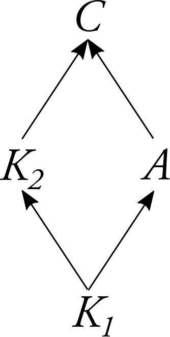
Here is a DAG representing the causal structure of Newcomb’s Problem:
There is a common cause, $K_1$, of both your action, $A$, and the prediction which has been made about your action, $K_2$. Your action and the prediction, $K_2$, will causally determine the amount of money which goes to charity, $C$. The variable $A$ can take on two values, $1$ and $2$. If $A=1$, then you take one box and leave money behind. If $A=2$, then you take both boxes, and don’t. Let’s similarly say that $K_1$ and $K_2$ can take on the values $1$ and $2$, and the variable $C$ can take on the values $1,010,000$, $1,000,000$, $10,000$, and $0$, depending upon how much money goes to charity.
One bit of terminology we’ll need: given a DAG, let’s say that the parents of a variable $V$, $\mathbf{PA}(V)$, are those variables which have a directed edge leading from them to $V$. Thus, in the DAG above, the parents of $C$, $\mathbf{PA}( C )$, are $A$ and $K_2$. Both $K_2$ and $A$ have a single parent, $K_1$. And $K_1$ doesn’t have any parents.
As I’ll use the term here, a causal Bayes net is a pair $< \mathbb{V}, \mathbb{E}, \Pr >$ of a DAG, and a probability function $\Pr$ defined over the values of the variables $V \in \mathbb{V}$, such that the probability function $\Pr$ satisfies the Markov Condition with respect to that DAG.
Markov Condition. A probability function $\Pr$ over the variables in $\mathbb{V} = \{ V_1, V_2, \dots, V_N \}$ satisfies the Markov Condition, relative to a given DAG $<\mathbb{V}, \mathbb{E}>$ if and only if
$$
\Pr(V_1, V_2, \dots, V_N) = \prod_i \Pr(V_i \mid \mathbf{PA}(V_i))
$$
For instance: if you want to know the probability that $K_1$ takes on the value $k_1$, $K_2$ takes on the value $k_2$, $A$ takes on the value $a$, and $C$ takes on the value $c$,
$$
\Pr(K_1 = k_1, K_2 = k_2, A=a, C=c)
$$
all you need to calculate this are the conditional probabilities $\Pr(C=c \mid K_2=k_2, A=a)$, $\Pr(K_2=k_2 \mid K_1=k_1)$, and $\Pr(A=a \mid K_1=k_1)$. Multiply them together, and you get $\Pr(K_1=k_1, K_2=k_2,A=a,C=c)$. In this way, the Markov Condition allows you to construct the entire joint probability function over $K_1, K_2, A,$ and $C$ from just knowledge of the conditional probabilities $\Pr(V \mid \mathbf{PA}(V))$. In Newcomb’s Problem, let’s say that those conditional probabilities are as follows:
\begin{align}
\Pr(K_1 = 1) &= 0.5 &\Pr(K_1 = 2)&= 0.5 \\\
\Pr(A=1 \mid K_1 = 1) &= 0.51 &\qquad \Pr(K_2 = 1 \mid K_1 = 1) &= 1 \\\
\Pr(A=2 \mid K_1 = 2) &= 0.51 &\qquad \Pr(K_2 = 2 \mid K_1 = 2) &= 1 \\\
\Pr(C=1,000,000 \mid A=1, K_2 = 1) &= 1 &\Pr(C=0 \mid A=1, K_2 = 2) &= 1 \\\
\Pr(C=1,010,000 \mid A=2, K_2 = 1) &= 1 &\Pr(C=10,000 \mid A=2, K_2 = 2) &= 1
\end{align}
There is another, equivalent, formulation of the Markov Condition which will be useful later on, so let me mention it briefly here:
Markov Condition (v2). A probability function $\Pr$ over the variables in $\mathbb{V} = \{ V_1, V_2, \dots, V_N \}$, satisfies the Markov Condition, relative to a given DAG $<\mathbb{V}, \mathbb{E}>$ if and only if, for any variable $V \in \mathbb{V}$, and any variable ${K}$ which is not causally downstream of $V$, $V$ and ${K}$ are probabilistically independent, conditional on $\mathbf{PA}(V)$
$$
\Pr(K \mid V, \mathbf{PA}(V)) = \Pr(K \mid \mathbf{PA}(V))
$$
Given the joint probability distribution, conditional probabilities can be calculated in the usual way via the ratio formula—$\Pr(X \mid Y) := \Pr(XY)/\Pr(Y)$ (so long as $\Pr(Y) \neq 0$). Conditionalization on $A$ will allow $A$ to provide information about $K_1$, which, in turn, will provide information about $K_2$. And it is exactly this kind of ‘backtracking’ information which the causal decision theorist wishes to exclude from their evaluation of an act. So, if we’re causal decision theorists, we won’t want to evaluate acts with a probability function conditioned on the act. With a DAG in hand, we are in a position to define up a causal probability function which filters out this kind of ‘backtracking’ information.
Causal Probability. Given a causal Bayes net $<\mathbb{V}, \mathbb{E}, \Pr>$, define the causal probability for $A=a$ as
$$
\Pr(V_1, V_2, \dots, V_N \mid\mid A=a) := \Pr(A \mid\mid A=a) \cdot \prod _{V \neq A} \Pr(V \mid \mathbf{PA}(V))
$$
and we stipulate that $\Pr(A=a \mid\mid A=a) = 1$.
That is: to get the causal probability for an act $A=a$, you take the factorization of $\Pr$ provided by the Markov Condition, and you simply replace the term for $\Pr(A \mid \mathbf{PA}(A))$ with a new term, $\Pr(A \mid\mid A=a)$, where we stipulate that the new term $\Pr(A \mid\mid A=a)$ takes the value $1$ if $A=a$ and otherwise takes the value $0$.
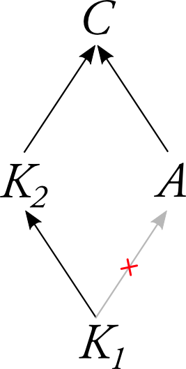
This causal probability will not obey the Markov Condition relative to our original DAG. However, it will obey the Markov Condition relative to an updated DAG in which you’ve removed the directed edges going into the variable $A$—call this the post-intervention DAG. For instance, given the original DAG from Newcomb’s Problem, the post-intervention DAG will be the one where we have removed the arrow leading from $K_1$ to $A$.
An intervention is a way of setting the value of a variable like $A$ which severs any causal influence between $A$ and its parents in the DAG. If you had intervened upon the variable $A$ to set its value to $a$, then the DAG shown in figure 2 would be the correct representation of the post-intervention causal structure. Moreover, relative to that post-intervention causal structure, the probability function $\Pr(-\mid\mid A=a)$ would satisfy the Markov Condition.
To think about these kinds of interventions more carefully, let’s include in our DAG of Newcomb’s Problem an explicit variable for whether the intervention on $A$ has taken place.
The new variable, $I_A$, can take on the values $0, 1,$ and $2$. If $I_A = 0$, then $A$ will take on the same value as $K_1$. If, however, $I_A = 1$, then $A$ will take on the value $1$, no matter what value $K_1$ takes on. And similarly, if $I_A = 2$, then $A$ will take on the value $2$, no matter what value $K_1$ takes on.
That is: the probability function over this new DAG has the same conditional probabilities for $K_1, K_2,$ and $C$ as the previous DAG, but the conditional probabilities for $A$ are now this:
\begin{align}
\Pr(A=1 \mid I_A = 0, K_1 = 1) &= 1 &\qquad \Pr(A=2 \mid I_A = 0, K_1 = 2) &= 1 \\\
\Pr(A=1 \mid I_A = 1, K_1 = 1) &= 1 &\qquad \Pr(A=1 \mid I_A = 1, K_1 = 2) &= 1 \\\
\Pr(A=2 \mid I_A = 2, K_1 = 1) &= 1 &\qquad \Pr(A=1 \mid I_A = 2, K_1 = 2) &= 1
\end{align}
Then, the probability function from our original DAG will just be this new probability function conditionalized upon $I_A=0$. And the probability function from the post-intervention DAG, $\Pr(- \mid\mid A=a)$, will just be this new probability function conditionalized upon $I_A = a$.
4. Interventions as Acts
Meek and Glymour use the tools of causal Bayes nets to formulate a version of causal decision theory which says that you should choose an act with maximal $U$-value, where
$$
U(A) = \sum_S \Pr(S \mid\mid A) \cdot V(SA)
$$
states are understood as assignments of values to the variables in $\mathbb{V}$, and the causal probabilities $\Pr(S \mid\mid A)$ are understood as the post-intervention probabilities defined in the previous section.
This is a fine theory for a causal decision theorist to accept. I don’t have any objection to Meek and Glymour attributing this theory to causal decision theorists; but I do have an objection to Meek and Glymour’s interpretation of this theory. For, on Meek and Glymour’s interpretation, the theory becomes a version of evidential decision theory.
First, Meek and Glymour object to the possibility of cases like Newcomb’s Problem, on the grounds that the case, as originally described, is not a true decision problem.
“We find something odd in questions about what an agent, no matter whether oneself or another, ought to do when one knows the agent’s action, whatever it is, will be necessitated by circumstances that cannot be influenced by any response to the question. Both advise and deliberation then seem pointless, and their benefits illusory.” (p. 1007)
Two comments on these remarks: firstly, in order to construct cases like Newcomb’s Problem, it needn’t be the case that your action is necessitated by past causal factors. For instance, in our original causal Bayes net of the case from the previous section, whether you take one box or two was not necessitated by the factor $K_1$ (since $\Pr(A=a \mid K_1 = a)$ was only 51%, not 100%), though $K_1$ did still causally influence your act. Secondly, and more importantly, in these remarks, Meek and Glymour are rejecting compatibilism about free will, saying that an agent cannot freely deliberate if their deliberation is itself caused. Perhaps this view is correct (well, it’s not, but let’s not dwell upon that right now), but if we accept this view, and if we accept what the Markov Condition has to say about the relationship between the world’s causal structure and the probability function $\Pr$, then we shouldn’t think that our acts can ever be probabilistically correlated with states of the world which are outside of our control. (For, to be clear, given the Markov Condition, the only way for an act to be correlated with a factor which isn’t causally downstream of it is for the act and the factor to have a common cause, which requires that the act be caused.)
That’s all to say: if you think cases like Newcomb’s Problem are genuine decision problems (decision problems in which you are free to undertake any act), then you had better think that our acts can be both free and caused. Which is to say: you had better be a compatibilist about free will.
Meek and Glymour continue:
“Even so, two possible reasons to deliberate or advise suggest themselves…You may wish to know…what someone otherwise like you but free to choose among alternative actions would rationally choose to do. Alternatively, one may view decisions…as the result of the action of a dual system with a default part and an extraordinary part—the default part subject to causes that may also influence the outcome through another mechanism, but the extraordinary part not so influenced and having the power to intervene and displace or modify the production of the default part. For brevity we will describe the extraordinary part as the Will.”
That is: Meek and Glymour suppose that the causal structure of Newcomb’s Problem is as shown in figure 2, where the intervention variable $I_A$ is the ‘extraordinary’ part—the Will—which is capable of overriding the ‘default’ behavior caused by $K_1$.
At this point, the case Meek and Glymour are considering is emphatically not the original Newcomb’s Problem (it is rather what Joyce (2018) calls a pseudo-Newcomb problem, as it fails to meet Joyce’s conditions $NP_1$ and $NP_4$, which any genuine Newcomb problem must meet). But let’s put that point to the side. Meek and Glymour are not considering Newcomb’s Problem, but this is an intentional choice, as they do not think that the case as usually understood constitutes a genuine decision problem. This is a philosophical disagreement between causal decision theorists and Meek and Glymour about whether free deliberation is compatible with the knowledge that one’s acts are caused—though it’s not a philosophical disagreement that I want to dwell upon here.
What I want to dwell upon here is instead the view that Meek and Glymour attribute to causal decision theorists when they write that:
“The causal decision theorist conditions on the event of an intervention, while the ‘evidential’ decision theorist conditions on an event…that is not an intervention. The difference in the two recommendations does not turn on any difference in normative principles, but rather on a substantive disagreement about the causal principles at work in the context of decision-making—the causal decision theorist thinks that when someone decides how to act, an intervention occurs, and the ‘evidential’ decision theorist thinks otherwise.” (p. 1009)
This is not an accurate characterization of the causal decision theorist’s position. The causal decision theorist does not think that, whenever you decide how to act, an intervention occurs.
One thing that is surely true of causal decision theorists is that they think the original Newcomb’s Problem is a counterexample to EDT. This case is the motivation for their theory. If it was already handled by EDT, there would be no need for CDT. But recall the Very Important Point from section 2: there is a difference between EDT and CDT only if there is a correlation between some factor outside of your control, $K$, and your act—that is, there is a difference between EDT and CDT only if, for some $K$,
$$
\Pr(K \mid A) \neq \Pr(K)
$$
But suppose that, whenever you choose an act, $A$, an intervention occurs. Since an intervention has occurred, $A$ does not have any causal parents (recall the post-intervention DAG from figure 2). So the Markov Condition (v2) tells us that your act must be probabilistically independent of all factors which are not causally downstream of it—and in particular, your act must be probabilistically independent of the prediction in Newcomb’s Problem. Thus, for any factor $K$ which is not causally downstream of your act—and, in particular, the prediction—it must be that
$$
\Pr(K \mid A) = \Pr(K)
$$
But then, EDT and CDT must give the same advice, and Newcomb’s Problem could not present a counterexample to EDT, unless it also presented a counterexample to CDT.
Meek and Glymour’s distinction between the default system and the Will suggests that perhaps they are thinking that a correlation exists between your choice and the prediction because of the default system, though, once you intervene with an act of the Will, such correlations will go away. In that case, Meek and Glymour may be interpreting the causal decision theorist as saying that you ought to intervene, and not allow your default system to choose for you. (Thoughts along these lines show up in Hitchcock (2016).)
This is also not an accurate characterization of the causal decision theorist’s position. The causal decision theorist attaches absolutely no value to interventions as such. Suppose that your default system is on a course to take both boxes. According to the causal decision theorist, what is the utility of letting the predictable default system run its course, $D$? It is (using the same notation from section 1)
\begin{align}
U(D) &= \Pr(M) \cdot V(MD) + \Pr(\neg M) \cdot V(\neg M D) \\\
&= 1,010,000 \cdot \Pr(M) + 10,000 \cdot \Pr(\neg M)
\end{align}
And what, according to the causal decision theorist, is the utility of intervening so as to bring it about that you take both boxes in a way which could not be predicted, $I$? It is also
\begin{align}
U(I) &= \Pr(M) \cdot V(MI) + \Pr(\neg M) \cdot V(\neg M I) \\\
&= 1,010,000 \cdot \Pr(M) + 10,000 \cdot \Pr(\neg M)
\end{align}
$\Pr(M \mid I)$ is higher than $\Pr(M \mid D)$—but, in evaluating acts, the causal decision theorist cares not at all about the probabilities of states of nature conditional on acts, $\Pr(K \mid A)$. Evaluating acts in this way leads to the irrational policy of ‘managing the news’ which the causal decision theorist seeks to avoid. They avoid irrationally managing the news by utilizing the unconditional probabilities of states of nature, $\Pr(K)$, when evaluating acts. The causal decision theorist is therefore indifferent between selecting two boxes in a predictable way and selecting two boxes in an unpredictable way. Being predictable does nothing to change the amount of money in front of you; it does nothing to improve the world; and therefore has nothing to speak in its favor, according to the causal decision theorist.
Evidential decision theorists, on the other hand, may attach quite a lot of value to interventions. For EDT, interventions are often far more chioceworthy than the default system. If your default system is on a course to take two boxes, so that $\Pr(M \mid D) = 0.49$, and intervening so as to take two boxes is less predictable, $\Pr(M \mid I) = 0.5$, then $V(D)$ will be $500,000$ as before, but
\begin{align}
V(I) &= \Pr(M \mid I) \cdot V(MI) + \Pr(\neg M \mid I) \cdot V(\neg MI) \\\
&= 0.5 \cdot 1,010,000 + 0.5 \cdot 10,000 \\\
&= 510,000
\end{align}
So the evidential decision theorist will advise you to intervene, so as to be less predictable.
Suppose that intervening with an act of the Will is to some extent dispreferred—you’d rather not think about what you’re doing, so intervening costs some small amount of value, $\epsilon$. Then, the view which Meek & Glymour call “causal decision theory” will advise you to intervene rather than let the default system choose two boxes, even though this act is causally dominated by allowing the default system to choose for you. For there are two possible states of nature: either there is a million dollars in box #1, $M$, or there is not, $\neg M$. If there is a million dollars in box #1, then allowing the default system to choose two boxes, $D$, has a higher value than intervening so as to take two boxes, $I$,
\begin{align}
V(M D) &= 1,010,000 &\qquad V(M I) &= 1,010,000 - \epsilon
\end{align}
And, if there is not a million dollars in box #1, then allowing the default system to choose two boxes has a higher value than intervening so as to take two boxes,
\begin{align}
V(\neg M D) &= 10,000 &\qquad V(\neg M I) &= 10,000 - \epsilon
\end{align}
Causal decision theorists accept a principle of causal dominance which says that causally dominated acts are irrational. So they do not recommend intervening in this case. So the view Meek & Glymour are calling ‘causal decision theory’ is not causal decision theory. (It is, instead, evidential decision theory.)
In sum: the position which Meek & Glymour attribute to causal decision theorists is a form of libertarianism about free will—the view that acts constitute interventions. Far from being central to CDT, this is actually a thesis which, if true, would render CDT unnecessary, since, if this thesis were true, CDT and EDT would never disagree. Nor does the causal decision theorist think that we ought to intervene, if we can. Intervention is worthless to the causal decision theorist. The view which evaluates acts differently, depending upon whether they are interventions or not, is evidential decision theory.
5. Interventions as Measures of Efficacy
As I said before, to some extent this is a terminological dispute about what is properly called “causal decision theory”. (It is equally, of course, an interpretive question about how to understand authors like Gibbard & Harper, Skyrms, Lewis, and Joyce—and, here, the barest modicum of charity militates against the Meek & Glymour interpretation.) But, more importantly, using the label “causal decision theory” for a version of evidential decision theory which utilizes causal Bayes nets obscures what is at issue in the debate between EDT and CDT, and what is at issue between one-boxers and two-boxers.
There is, of course, a very interesting philosophical debate about whether we have libertarian free will—whether our acts constitute interventions—and whether it makes sense to deliberate about what to do while knowing that your decision is caused by factors outside of your control. But this is not the debate between one-boxers and two-boxers. Both one-boxers and two-boxers agree that Newcomb’s Problem is a genuine decision problem. What they disagree about is how to act in that decision problem. But if deliberation is impossible or pointless when you believe your acts are caused, or if all acts are interventions, then Newcomb’s Problem would not be a genuine decision problem.
Both one-boxers and two-boxers accept that there may be correlations between your choice and states over which you exercise no control, and that you may freely deliberate in such circumstances. So both one-boxers and two-boxers accept that not all acts are interventions, and that deliberation does not lose its point when this is so. What is at issue between them is whether correlations between your act and good states outside of your control speak in favor of that act. The one-boxer says “yes”, while the two-boxer says “no”. The two-boxer thinks that you should choose acts which do the most possible to improve the world in which you find yourself, whatever bad news those acts may carry with them.
So the two-boxer wishes to evaluate acts by looking at the good they stand to promote, and not considering the good those acts stand to merely indicate. And it is here that the causal probabilities supplied by interventions will be of interest to the causal decision theorist. They may want to use the causal probabilities $\Pr(S \mid\mid A)$ as a measure, not of the probability of $S$, given that $A$ is performed, but rather as a measure of $A$'s ability to bring $S$ about—that is, as a measure of $A$'s efficacy in promoting the state $S$. What the causal decision theorist says is that you should evaluate an act $A$ by using causal probabilities, whether the act $A$ is an intervention or not.
Let’s distinguish acts which are the results of interventions by the Will (unpredictable acts) from those which are not (predictable acts). If $A$ is a predictable act, let ‘$I_A$’ be an intervention which has the same causal consequences as $A$, but which is (because an intervention) unpredictable. The evidential decision theorist will treat $A$ and $I_A$ differently.
Evidential Decision Theory. The choiceworthiness of $A$ is given by
$$
V(A) = \sum_S \Pr(S \mid A) \cdot V(SA)
$$
Whereas the choiceworthiness of $I_A$ is given by
\begin{align}
V(I_A) &= \sum_S \Pr(S \mid I_A) \cdot V(S I_A) \\\
&= \sum_S \Pr(S \mid\mid A) \cdot V(SA)
\end{align}
(In the above, think of $S$ as an assignment of values to the variables in the DAG. Also note that I assume you don’t take the intervention $I_A$ to be intrinsically valuable, so that $V(S I_A) = V(S A)$.) On the other hand, since the causal decision theorist evaluates all acts using the causal probabilities $\Pr(S \mid\mid A)$ as measures of causal strength, CDT treats $A$ and $I_A$ in precisely the same way.
Causal Decision Theory. The choiceworthiness of $A$ is given by
$$
U(A) = \sum_S \Pr(S \mid\mid A) \cdot V(SA)
$$
And the choiceworthiness of $I_A$ is given by
\begin{align}
U(I_A) &= \sum_S \Pr(S \mid\mid I_A) \cdot V(S I_A) \\\
&= \sum_S \Pr(S \mid\mid A) \cdot V(SA)
\end{align}
In sum, Meek and Glymour present causal decision theory as though it treats $A$ and $I_A$ differently. But it emphatically does not. The view they are discussing is evidential decision theory. It is a version of EDT which makes use of tools from causal modeling—in particular, the notion of an intervention and the Markov Condition—to specify the available acts and the relevant probability function. But, once the available acts are specified and probability function given, the view they are calling “causal decision theory” gives precisely the same advice which EDT would give with that choice of acts and that probability function.
This is to some extent a question about which view is most deserving of the name “causal decision theory” (and, on this score, I would have hoped it obvious that the view introduced and defended by authors like Gibbard & Harper, Skyrms, Lewis, and Joyce under the name “causal decision theory” is more deserving of the name than the view those authors were attempting to argue against), but there is also a deeper issue with using terminology in this way. Because the view called “causal decision theory” by Meek & Glymour evaluates acts by the goods they indicate, this terminological choice serves to obscure the central lesson which causal decision theorists draw from Newcomb’s Problem—namely, that acts should be evaluated by the good they promote, and not the good they merely indicate.
2017, Jun 25
The Impossibility of a Paretian Liberal
A foundational assumption in welfare economics is that, if everyone prefers A to B, then A is better than B. This normative claim is called the ‘weak Pareto principle’. At a first glance, this principle can appear unimpeachable. At the very least, it appears to be a sensible principle for policy makers to adopt.
Many of us are also committed to the principle that there are some choices that should be left up to the individual. Even if everyone else prefers that my nose be pierced, if I prefer it unpierced, then it is better for my nose to remain unpierced. A state-of-affairs in which I am compelled to pierce my nose, against my wishes, is worse than a state-of-affairs in which I get to make up my own mind about whether my nose is pierced. And that’s so no matter how many other people would prefer to see me with a pierced nose. Call this committment ‘minimal liberalism’.
In 1970, Amartya Sen produced an amazing result which seems to show that minimal liberalism and the weak Pareto principle are inconsistent with one another. Today I want to rehearse Sen’s result, and introduce an objection to Sen’s way of formalizing ‘minimal liberalism’ first made by Allan Gibbard. I think that Gibbard’s objection teaches us that Sen formulated liberalism incorrectly. However, I’ll conclude by showing that a better formulation of liberalism, one that avoids Gibbard’s objection, is also inconsistent with the weak Pareto principle.
The Impossibility of a Paretian Liberal, take 1
Sen’s result relies upon a formal framework in which we think of social goodness as determined by the preferences of the individuals living in a society. So we suppose that all the members of our society have their own preference ordering over state-of-affairs. Individual $i$ has the preference ordering $\succeq_i$. That’s a weak preference ordering; I’ll assume that we can get a strong perference ordering $\succ_i$ out of a weak one through the definition $A \succ_i B := A \succeq_i B \wedge B \not\succeq_i A$.
Given the preferences of every individual, $\succeq_i$, a social welfare function $W$ delivers a group preference ordering, $\succeq_G$, which tells us which states-of-affairs the group prefers to which other state-of-affairs.
An implicit normative assumption is that we may treat the group preference ordering as a betterness ordering. That is: if $A \succ_G B$, then $A$ is better than $B$. So we can think of the subscripted ‘$G$’ as standing either for ‘group’ or for ‘goodness’. (I’ll also assume throughout, by the way, that the social welfare function $W$ will always be defined, no matter which collection of individual preference orderings we hand it.)
Sen then interprets the weak Pareto principle and minimal liberalism in terms of this social welfare function. In these terms, the weal Pareto principle says that, if everyone prefers $A$ to $B$, then the group must prefer $A$ to $B$. And minimal liberalism says that every person is decisive with respect to some choice. That is: every person has at least one pair of options such that, whatever that person’s preferences are between those two options, that becomes the group’s preference. If I prefer my nose being pierced to my nose not being pierced, then that’s what the group prefers, too. And if I prefer my nose not being pierced to my nose being pierced, then that’s what the group prefers.
Weak Pareto Principle
If $A \succ_i B$ for all $i$, then $A \succ_G B$.
Minimal Liberalism
For all $i$, there is at least one pair of alternatives, $A$ and $B$, such that, if $A \succ_i B$, then $A \succ_G B$ and, if $B \succ_i A$, then $B \succ_G A$.
Sen additionally assumes that, if we’re going to interpret $\succeq_G$ as a social betterness ordering, then it had better not land us in cycles. That is, it had better not tell us that $A$ is better than $B$, $B$ is better than $C$, and $C$ is better than $A$.
No Cycles
There is no sequence of states-of-affairs $A_1, A_2, \dots, A_N$ such that
$$
A_1 \succ_G A_2 \succ_G \dots \succ_G A_N \succ_G A_1
$$
Sen then proves that there is no social welfare function which satisfies Weak Pareto Principle, Minimal Liberalism, and No Cycles. I won’t go through the formal proof here; but I’ll go through a nice illustrative example from Sen (cultural references have been updated).
Prude is outraged and offended by Fifty Shades of Gray. Lewd, on the other hand, is delighted by the book. Prude would most prefer that nobody read the filth. However, if somebody must read it, Prude would rather read it himself than expose a libertine like Lewd to its influence. Lewd would most prefer that both he and Prude read the book. However, if only one of them is to read it, Lewd would rather it be Prude—he relishes the thought of Prude’s horrified reactions.
Thus, Prude and Lewd’s preference orderings are given in the following table.
Prude
Lewd
1st.
Neither reads ($N$)
Both read ($B$)
2nd.
Prude reads ($P$)
Prude reads ($P$)
3rd.
Lewd reads ($L$)
Lewd reads ($L$)
4th.
Both read ($B$)
Neither reads ($N$)
For the purposes of illustration, suppose that Prude and Lewd are the only people in this society. And let’s suppose that whether you read a book is a matter which ought to be left up to the individual. If you prefer to read, then it’s better that you read; if you prefer to not read, then it’s better that you refrain. That’s all we need to bring out the conflict between Weak Pareto Principle, Minimal Liberalism, and No Cycles.
The only difference between $P$ and $N$ is whether Prude reads. It should be entirely up to Prude whether he read or not. Since he prefers to not read, Minimal Liberalism tells us that it is better if he doesn’t. So
$$
N \succ_G P
$$
Note that both Prude and Lewd prefer $P$ to $L$. So, by the Weak Pareto Principle,
$$
P \succ_G L
$$
And, the only difference between $L$ and $N$ is whether Lewd reads. It should be entirely up to Lewd whether he read or not. Since he prefers to read, Minimal Liberalism tells us that it is better if he does. So
$$
L \succ_G N
$$
But now we’ve violated No Cycles.
$$
N \succ_G P \succ_G L \succ_G N
$$
So it seems that we face a choice: either reject the Weak Pareto Principle, or reject Minimal Liberalism. You can’t be both a Paretian and a liberal. If you want to be a liberal, you’d better reject the Weak Pareto principle.
The Impossibility of a Liberal?
Actually, matters are worse. Even rejecting the Weak Pareto Principle won’t get you out of trouble. Allan Gibbard showed that Minimal Liberalism leads to cycles all by itself, even without the Weak Pareto Principle.
Consider Match and Clash. Clash is a non-conformist. She would prefer having a pierced nose, but what’s most important to her is that her fashion be different from Match’s. So she wants to pierce her nose if (but only if) Match doesn’t pierce hers. Match is a follower. She doesn’t want to pierce her nose, but she does want her fashion to match Clash’s. So she wants to pierce her nose if (and only if) Clash pierces hers. Therefore, Clash and Match’s preferences are given by the following table.
Clash
Match
1st.
Clash pierces ($C$)
Neither pierce ($N$)
2nd.
Match pierces ($M$)
Both pierce ($B$)
3rd.
Both pierce ($B$)
Clash pierces ($C$)
4th.
Neither pierce ($N$)
Match pierces ($M$)
For the purposes of illustration, let’s suppose that Match and Clash are the only people in this society. And Let’s suppose that whether your nose is pierced is the kind of thing which ought to be left up to the individual. If you prefer a pierced nose, then it’s better if your nose is pierced. And if you don’t, then it’s better if it’s not pierced.
Note that the only difference between $C$ and $N$ is whether Clash pierces. And Clash prefers $C$ to $N$. So the liberal says that $C$ is better than $N$.
$$
C \succ_G N
$$
The only difference between $N$ and $M$ is whether Match pierces. And Match prefers $N$ to $M$. So the liberal says that $N$ is better than $M$.
$$
N \succ_G M
$$
The only difference between $M$ and $B$ is whether Clash pierces. And Clash prefers $M$ to $B$. So the liberal says that $M$ is better than $B$.
$$
M \succ_G B
$$
And, finally, the only difference between $B$ and $C$ is whether Match pierces. Since Match prefers $B$ to $C$, the liberal says that $B$ is better than $C$.
$$
B \succ_G C
$$
But now we’ve contradicted No Cycles.
$$
C \succ_G N \succ_G M \succ_G B \succ_G C
$$
So Minimal Liberalism is inconsistent with No Cycles all by itself. We didn’t have to bring up the Weak Pareto Princple at all.
The Impossibility of a Paretian Liberal, take 2
Sen’s principle Minimal Liberalism assumes that the right way to think about liberalism is in terms of the decisiveness of individual preference. Sen’s liberal thinks that, if Prude prefers to not read, then it’s better if Prude not read (all else equal). And, if Lewd prefers to read, then it’s better if Lewd read (again, all else equal). What Gibbard’s case shows us, I think, is that this way of understanding liberalism is misguided.
And, in retrospect, we should recognize that we ought to have rejected Minimal Liberalism as a characterization of liberalism on independent grounds. Liberals think that certain self-regarding decisions should be left up to the individual. One of Mill’s arguments for this was that the individual is in a better position to know what’s best for them than the rest of society. However, Mill didn’t think that individuals were necessarily right about what’s in their own best interest.
Liberals should acknowledge that people can and do make self-regarding choices that make them worse off. A libertine liberal like Lewd will grant that what Prude reads should be left up to him. But that won’t keep Lewd from thinking that Prude’s diet of religious drivel is making his life worse. And surely Lewd should also think that, all else equal, it’s better for people’s lives to go better, and worse for them to go worse.
So the liberal shouldn’t think that, when it comes to self-regarding decisions, people’s actual preferences are objectively best. What they should think is that, when it comes to self-regarding decisions, it is better to allow people to choose for themselves than for the state to choose for them. That is: the liberal ought to think that, when it comes to self-regarding decisions, it is worse to deprive people of liberty than it is to allow them to make their own poor choices.
(At least, this is what a consequentialist liberal ought to think—though a non-consequentialist liberal is free to admit that things would be better if people were compelled to make the right choices, though such an arrangement would be unjust in spite of its betterness. I’m very sympathetic to this kind of position, but I’ll put it aside for the nonce.)
Our earlier discussion did not draw any distinction between possibilities in which people were forced to take certain options and those in which they freely chose those options. Let’s introduce this distinction, and use it to formulate our principle of liberalism.
Liberalism as Non-Compulsion does not fall prey to Gibbard-style objections. It is easy to see that the principle on its own could never give rise to cycles of betterness. The set of all possible states-of-affairs is partitioned by those in which all self-regarding choices are free and those in which some self-regarding choice is not free. And all Liberalism as Non-Compulsion says is that everything in the former set is better than everything in the latter set. On its own, this won’t lead to a cycle.
However, conjoined with the Weak Pareto Principle, this new principle of liberalism does run into cycles, in precisely the same way as before.
Let’s return to Sen’s example of Prude and Lewd. First, we’ll distinguish between those possibilities in which all choices are free and those possibilities in which some choices are compelled. We’ll subscript each of the previous states-of-affairs with an ‘$F$’ if they are states-of-affairs in which all choices are free and with a ‘$C$’ if it is a state-of-affairsin which people are compelled against their will to act in a certain way.
$N_F$: Both Prude and Lewd freely choose to not read.
$N_C$: Both Prude and Lewd are forced to not read.
$L_F$: Lewd freely chooses to read and Prude freely chooses to not read.
$L_C$: Lewd is forced to read, and Prude is forced to not read.
$P_F$: Prude freely chooses to read and Lewd freely chooses to not read.
$P_C$: Prude is forced to read and Lewd is forced to not read.
$B_F$: Both Prude and Lewd freely choose to read.
$B_C$: Both Prude and Lewd are forced to read.
Now suppose that, while both Prude values freedom—so that, all else equal, he would rather have Lewd and himself choose freely than be compelled—he values it less than he does keeping the filth of Fifty Shades from spreading. And, while Lewd values freedom—so that, all else equal, he would rather have Prude and himself choose freely than be compelled—he values it less than Prude’s disgust, and his delight, at the book’s depravity. So, if we ignore the subscripts, their preferences are the same as before, and otherwise, each of them prefers outcomes where choices are free.
Prude
Lewd
1st.
$N_F$
$B_F$
2nd.
$N_C$
$B_C$
3rd.
$P_F$
$P_F$
4th.
$P_C$
$P_C$
5th.
$L_F$
$L_F$
6th.
$L_C$
$L_C$
7th.
$B_F$
$N_F$
8th.
$B_C$
$N_C$
Now, by Liberalism as Non-Compulsion, the outcome where Lewd freely chooses to read and Prude freely refrains is better than the outcome where Prude is forced to read and Lewd to refrain.
$$
L_F \succ_G P_C
$$
But both Prude and Lewd prefer $P_C$ to $L_F$. So, by the Weak Pareto Principle,
$$
P_C \succ_G L_F
$$
And this contradicts No Cycles.
$$
L_F \succ_G P_C \succ_G L_F
$$
In sum: Gibbard showed us that we ought to reformulate Sen’s Minimal Liberalism. However, the best reformulation doesn’t get us out of the conflict with the Weak Pareto Principle. So the conflict is genuine. If you are a liberal, you cannot be a Paretian. If you are a liberal, you should deny that people’s preferences determine goodness in the way that Pareto imagined. If you are a Paretian, then you cannot be a liberal. If you are a Paretian, you should deny that it’s always best for self-regarding decisions to be left to the individual.